Download
1 / 33
360 likes | 695 Views
Fast Fourier Transform. A bunch of smart people. Outline (hopefully). Finite discrete signals Linear shift-invariant filters Impulse responses Circular convolutions Discrete Fourier Transform The Fast Fourier Transform. Continuous signals. Finite signals.

E N D
Fast Fourier Transform A bunch of smart people
Outline (hopefully) • Finite discrete signals • Linear shift-invariant filters • Impulse responses • Circular convolutions • Discrete Fourier Transform • The Fast Fourier Transform
Finite signals • Usually come from regular discretization
Finite signals • Usually come from regular discretization • Might as well think of them as vectors!
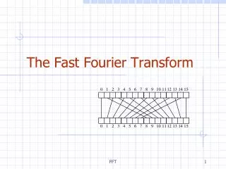
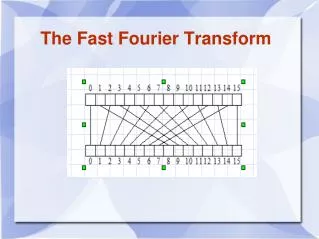
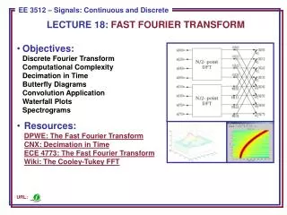
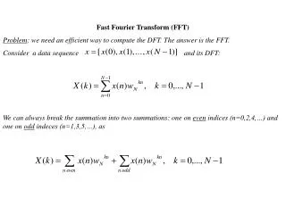
Discrete Fourier Transform Complexity O(N2) FFT is just an O(N log N) algorithm
Linear (i.e., matrices) Transformations on vectors
Transformations on vectors Linear (i.e., matrices) Shift invariant (in a circular way)
Closer look at shift invariance L is shift invariant iff
is the canonic basis for plays the role of Dirac's delta or impulse The canonic basis of RN
How does matrix L look like? h is the impulse response of L It captures all information about L!
How do we multiply L by v? This is why we care about convolutions!
The circular convolution Complexity O(N2)
What we have so far • We discretized a continuous function turning it into a vector in RN • We defined a class of transformations from RN to RN that we care about • Each linear shift-invariant transformations L can be written as a circular convolution • The convolution is with the impulse response h of the transformation L • We can compute it in O(N2)
This is too abstract! • Want to make a recording of your voice sound as if you were inside a bathroom? • Your bathroom transform sound in a linear, shift invariant way. • Record the sound of a clap in the bathroom. • Record your voice outside. • Convolve the two signals!
Easy to do in Matlab a = wavread('bathroom-ip.wav'); b = wavread('laugh.wav'); a = a / max(abs(a)); b = b / max(abs(b)); c = conv(a, b); c = c / max(abs(c)); p = audioplayer(c, 44000); play(p, [1 length(c)])
But first... Better convolution strategy O(N2) v Lv convolution FFT IFFT F-1LF F-1v O(N) F-1v product
Diagonalizing L • Need a basis of eigenvectors for L. Trick is to look at P first! • Assume for now that P has distinct eigenvalues. • If wi is an eigenvector of P, then it is also an eigenvector of L! • Lwiis an eigenvector of P, with the same eigenvalue • We must have • wiis also eigenvector of L (for some other eigenvalue) • Since P has a full set of wi, L is diagonalized by the same wi!
The eigenvalues of P Indeed, P has a full set!
Better convolution strategy O(N2) v Lv convolution FFT IFFT F-1LF F-1v O(N) F-1v product Not only does F exist. It does not depend on L!
We can also verify that... How do F and F-1 look like?
Finally!!! How to compute F-1v?
The eigenvalues of L Finally!!!
Discrete Fourier Transform FFT is just an O(N log N) algorithm
Better convolution strategy O(N2) v Lv convolution FFT IFFT F-1LF F-1v O(N) F-1v product
Fast Fourier Transform • Coley and Tukey, 1965 • Gauss, 1805
Better convolution strategy O(N2) v Lv convolution FFT IFFT F-1LF F-1v O(N) F-1v product
Easy to do in Matlab a = wavread('bathroom-ip.wav'); b = wavread('laugh.wav'); a = a / max(abs(a)); b = b / max(abs(b)); c = fftfilt(a, b); c = c / max(abs(c)); p = audioplayer(c, 44000); play(p, [1 length(c)])