Fast Fourier Transform

1. Fast Fourier Transform • Jean Baptiste Joseph Fourier (1768-1830) These lecture slides are adapted from CLRS.

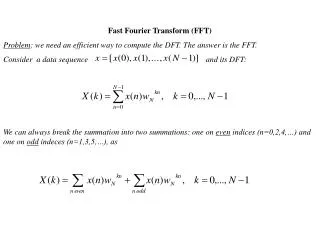
2. Fast Fourier Transform • Applications. • Perhaps single algorithmic discovery that has had the greatest practical impact in history. • Optics, acoustics, quantum physics, telecommunications, systems theory, signal processing, speech recognition, data compression. • Progress in these areas limited by lack of fast algorithms. • History. • Cooley-Tukey (1965) revolutionized all of these areas. • Danielson-Lanczos (1942) efficient algorithm. • Runge-König (1924) laid theoretical groundwork. • Gauss (1805, 1866) describes similar algorithm. • Importance not realized until advent of digital computers.

3. Polynomials: Coefficient Representation • Degree n polynomial. • Addition: O(n) ops. • Evaluation: O(n) using Horner's method. • Multiplication (convolution): O(n2).

4. Polynomials: Point-Value Representation • Degree n polynomial. • Uniquely specified by knowing p(x) at n different values of x. y = p(x) yj xj x

5. Polynomials: Point-Value Representation • Degree n polynomial. • Addition: O(n). • Multiplication: O(n), but need 2n points. • Evaluation: O(n2) using Lagrange's formula.

6. Best of Both Worlds • Can we get "fast" multiplication and evaluation? • Yes! Convert back and forth between two representations. Representation Multiplication Evaluation coefficient O(n2) O(n) point-value O(n) O(n2) FFT O(n log n) O(n log n) coefficient multiplication O(n2) interpolationinverse FFT evaluationFFT O(n log n) O(n log n) point-value multiplication O(n)

7. Converting Between Representations: Naïve Solution • Evaluation (coefficient to point-value). • Given a polynomial p(x) =a0 + a2x1 + . . . + an-1 xn-1, choose n distinct points {x0, x1, . . . , xn-1 } and compute yk = p(xk), for each k using Horner's method. • O(n2). • Interpolation (point-value to coefficient). • Given n distinct points {x0, x1, . . . , xn-1 } and yk = p(xk), compute the coefficients {a0, a1, . . . , an-1 } by solving the following linear system of equations. • Note Vandermonde matrix is invertible iff xk are distinct. • O(n3).

8. Fast Interpolation: Key Idea • Key idea: choose {x0, x1, . . . , xn-1 } to make computation easier! • Set xk = xj?

9. Fast Interpolation: Key Idea • Key idea: choose {x0, x1, . . . , xn-1 } to make computation easier! • Set xk = xj? • Use negative numbers: set xk = -xj so that (xk )2 = (xj )2. • set xk = -xn/2 + k • E = peven(x2) = a0 + a2172 + a4174 + a6176 + . . . + an-217n-2 • O = x podd(x2) = a117 + a3173 + a5175 + a7177 + . . . + an-117n - 1 • y0 = E + O, yn/2 = E - O

10. Fast Interpolation: Key Idea • Key idea: choose {x0, x1, . . . , xn-1 } to make computation easier! • Set xk = xj? • Use negative numbers: set xk = -xj so that (xk )2 = (xj )2. • set xk = -xn/2 + k • Use complex numbers: set x k = k where is nth root of unity. • (xk )2 = (-xn/2 + k )2 • (xk )4 = (-xn/4 + k )4 • (xk )8 = (-xn/8 + k )8

11. Roots of Unity • An nth root of unity is a complex number z such that zn = 1. •  = e 2 i / n = principal n th root of unity. • e i t = cos t + i sin t. • i2 = -1. • There are exactly n roots of unity: k, k = 0, 1, . . . , n-1. 2 = i 3 1 4 = -1 0 = 1 7 5 6 = -i

12. Roots of Unity: Properties • L1: Let  be the principal nth root of unity. If n > 0, then n/2= -1. • Proof:  = e 2 i / n n/2 = e  i = -1. (Euler's formula) • L2: Let n > 0 be even, and let  and  be the principal nth and (n/2)th roots of unity. Then (k ) 2 =  k . • Proof: (k ) 2 = e (2k)2 i / n= e (k) 2 i / (n / 2) =  k . • L3: Let n > 0 be even. Then, the squares of the n complex nth roots of unity are the n/2 complex (n/2) th roots of unity. • Proof: If we square all of the nth roots of unity, then each (n/2) th root is obtained exactly twice since: • L1  k + n / 2 = - k • thus, (k + n / 2) 2 = (k ) 2 • L2  both of these =  k • k + n / 2 and k have the same square

13. Divide-and-Conquer • Given degree n polynomial p(x) = a0 + a1x1 + a2 x2 + . . . + an-1 xn-1. • Assume n is a power of 2, and let  be the principal n th root of unity. • Define even and odd polynomials: • peven(x) := a0 + a2x1 + a4x2 + a6x3 + . . . + an-2 xn/2 - 1 • podd(x) := a1 + a3x1 + a5x2 + a7x3 + . . . + an-1 xn/2 - 1 • p(x) = peven(x2) + x podd(x2) • Reduces problem of • evaluating degree n polynomial p(x) at 0, 1, . . . , n-1 to • evaluating two degree n/2 polynomials at: (0)2, (1)2, . . . , (n-1)2 . • L3  peven(x) and podd(x) only evaluated at n/2 complex (n/2) th roots of unity.

14. FFT Algorithm if (n == 1) // n is a power of 2 return a0  e 2 i / n (e0,e1,e2,...,en/2-1)  FFT(n/2, a0,a2,a4,...,an-2) (d0,d1,d2,...,dn/2-1)  FFT(n/2, a1,a3,a5,...,an-1) for k = 0 to n/2 - 1 yk  ek + kdk yk+n/2 ek - kdk return (y0,y1,y2,...,yn-1) FFT (n, a0, a1, a2, . . . , an-1) O(n) complex multiplies if we pre-compute k.

15. Recursion Tree a0, a1, a2, a3, a4, a5, a6, a7 a0, a2, a4, a6 a1, a3, a5, a7 a0, a4 a2, a6 a3, a7 a1, a5 a0 a4 a2 a6 a1 a5 a3 a7 "bit-reversed" order

16. Proof of Correctness • Proof of correctness. Need to show yk = p(k ) for each k = 0, . . . , n-1, where  is the principaln th root of unity. • Base case. n = 1   = 1. Algorithm returns y0 = a0 = a0 0 . • Induction step. Assume algorithm correct for n / 2. • let  be the principal (n/2) throot of unity • ek = peven(k )= peven(2k )by Lemma 2 • dk = podd(k ) = podd(2k )by Lemma 2 • recall p(x) = peven(x2) + x podd(x2)

17. Best of Both Worlds • Can we get "fast" multiplication and evaluation? • Yes! Convert back and forth between two representations. Representation Multiplication Evaluation coefficient O(n2) O(n) point-value O(n) O(n2) FFT O(n log n) O(n log n) coefficient multiplication O(n2) evaluationFFT interpolationinverse FFT O(n log n) O(n log n) point-value multiplication O(n)

18. Inverse FFT • Forward FFT: given {a0, a1, . . . , an-1 } , compute {y0, y1, . . . , yn-1 } . • Inverse FFT: given {y0, y1, . . . , yn-1 } compute {a0, a1, . . . , an-1 }.

19. Inverse FFT • Great news: same algorithm as FFT, except use -1 as "principal" nth root of unity (and divide by n).

20. Inverse FFT: Proof of Correctness • Summation lemma. Let  be a primitive n th root of unity. Then • If k is a multiple of n then k = 1. • Each nth root of unity k is a root ofxn - 1 = (x - 1) (1 + x + x2 + . . . + xn-1),if k 1 we have: 1 + k + k(2) + . . . + k(n-1) = 0. • Claim: Fn and Fn-1 are inverses.

21. Inverse FFT: Algorithm if (n == 1) // n is a power of 2 return a0  e-2i/n (e0,e1,e2,...,en/2-1)  FFT(n/2, a0,a2,a4,...,an-2) (d0,d1,d2,...,dn/2-1)  FFT(n/2, a1,a3,a5,...,an-1) for k = 0 to n/2 - 1 yk (ek + kdk ) / n yk+n/2 (ek - kdk ) / n return (y0,y1,y2,...,yn-1) IFFT (n, a0, a1, a2, . . . , an-1)

22. Best of Both Worlds • Can we get "fast" multiplication and evaluation? • Yes! Convert back and forth between two representations. Representation Multiplication Evaluation coefficient O(n2) O(n) point-value O(n) O(n2) FFT O(n log n) O(n log n) coefficient multiplication O(n2) evaluationFFT O(n log n) interpolationinverse FFT O(n log n) point-value multiplication O(n)

23. Integer Arithmetic • Multiply two n-digit integers: a = an-1 . . . a1a0 and b = bn-1 . . . b1b0. • Form two degree n polynomials. • Note: a = p(10), b = q(10). • Compute product using FFT in O(n log n) steps. • Evaluate r(10) = a  b. • Problem: O(n log n) complex arithmetic steps. • Solution. • Strassen (1968): carry out arithmetic to suitable precision. • T(n) = O(n T(log n))  T(n) = O(n log n (log log n)1+ ) • Schönhage-Strassen (1971): use modular arithmetic. • T(n) = O(n log n log log n)

24. Extra Slides

25. Polynomials: Representation and Addition • Degree n polynomial. • Coefficient representation. • Point-value representation. • Addition. • O(n) for either representation.

26. Polynomials: Evaluation and Multiplication • Multiplication (convolution). • Brute force.O(n2). • Use 2n points.O(n). • Evaluation. • Horner's method.O(n). • Lagrange's formula.O(n2).