Download
1 / 16
190 likes | 423 Views
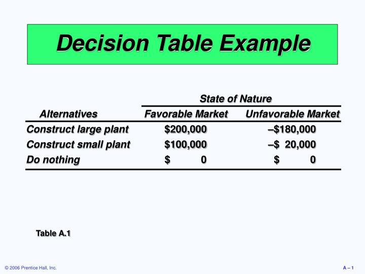
State of Nature Alternatives Favorable Market Unfavorable Market Construct large plant $200,000 –$180,000 Construct small plant $100,000 –$ 20,000 Do nothing $ 0 $ 0. Decision Table Example. Table A.1. EMV for node 1 = $10,000.

E N D
State of Nature Alternatives Favorable Market Unfavorable Market Construct large plant $200,000 –$180,000 Construct small plant $100,000 –$ 20,000 Do nothing $ 0 $ 0 Decision Table Example Table A.1
EMV for node 1 = $10,000 = (.5)($200,000) + (.5)(-$180,000) Payoffs Favorable market (.5) $200,000 1 Unfavorable market (.5) -$180,000 Construct large plant Favorable market (.5) $100,000 Construct small plant 2 Unfavorable market (.5) -$20,000 Do nothing EMV for node 2 = $40,000 = (.5)($100,000) + (.5)(-$20,000) $0 Decision Tree Example Figure A.2
States of Nature Favorable Unfavorable Alternatives Market Market Construct large plant (A1) $200,000 -$180,000 Construct small plant (A2) $100,000 -$20,000 Do nothing (A3) $0 $0 Probabilities .50 .50 EMV Example Table A.3 EMV(A1) = (.5)($200,000) + (.5)($180,000) = $10,000 EMV(A2) = (.5)($100,000) + (.5)($20,000) = $40,000 EMV(A3) = (.5)($0) + (.5)($0) = $0 Best Option
States of Nature Favorable Unfavorable Maximum Minimum Row Alternatives Market Market in Row in Row Average Constructlarge plant$200,000 -$180,000 $200,000 -$180,000 $10,000 Constructsmall plant$100,000 -$20,000 $100,000 -$20,000 $40,000 Do nothing$0 $0 $0 $0 $0 Maximax Maximin Equally likely Uncertainty Example Maximax choice is to construct a large plant Maximin choice is to do nothing Equally likely choice is to construct a small plant
Expected value under certainty = ($200,000)(.50) + ($0)(.50) = $100,000 EVPI Example The best outcome for the state of nature “favorable market” is “build a large facility” with a payoff of $200,000. The best outcome for “unfavorable” is “do nothing” with a payoff of $0.
Expected value under certainty Maximum EMV EVPI = – EVPI Example The maximum EMV is $40,000, which is the expected outcome without perfect information. Thus: = $100,000 – $40,000 = $60,000 The most the company should pay for perfect information is $60,000
The Decision Process in Operations Clearly define the problems and the factors that influence it Develop specific and measurable objectives Develop a model Evaluate each alternative solution Select the best alternative Implement the decision and set a timetable for completion
Risk • Each possible state of nature has an assumed probability • States of nature are mutually exclusive • Probabilities must sum to 1 • Determine the expected monetary value (EMV) for each alternative
Expected value under certainty Maximum EMV EVPI = – Expected Value of Perfect Information EVPI is the difference between the payoff under certainty and the payoff under risk
Decision Trees • Information in decision tables can be displayed as decision trees • A decision tree is a graphic display of the decision process that indicates decision alternatives, states of nature and their respective probabilities, and payoffs for each combination of decision alternative and state of nature • Appropriate for showing sequential decisions
Decision Trees Define the problem Structure or draw the decision tree Assign probabilities to the states of nature Estimate payoffs for each possible combination of decision alternatives and states of nature Solve the problem by working backward through the tree computing the EMV for each state-of-nature node
Complex Decision Tree Example Figure A.3
Complex Example Given favorable survey results EMV(2) = (.78)($190,000) + (.22)(-$190,000) = $106,400 EMV(3) = (.78)($90,000) + (.22)(-$30,000) = $63,600 The EMV for no plant = -$10,000 so, if the survey results are favorable, build the large plant
Complex Example Given negative survey results EMV(4) = (.27)($190,000) + (.73)(-$190,000) = -$87,400 EMV(5) = (.27)($90,000) + (.73)(-$30,000) = $2,400 The EMV for no plant = -$10,000 so, if the survey results are negative, build the small plant
Complex Example Compute the expected value of the market survey EMV(1) = (.45)($106,400) + (.55)($2,400) = $49,200 If the market survey is not conducted EMV(6) = (.5)($200,000) + (.5)($180,000) = $10,000 EMV(7) = (.5)($100,000) + (.5)(-$20,000) = $40,000 The EMV for no plant = $0 so, given no survey, build the small plant