Models to Represent the Relationships Between Variables (Regression)

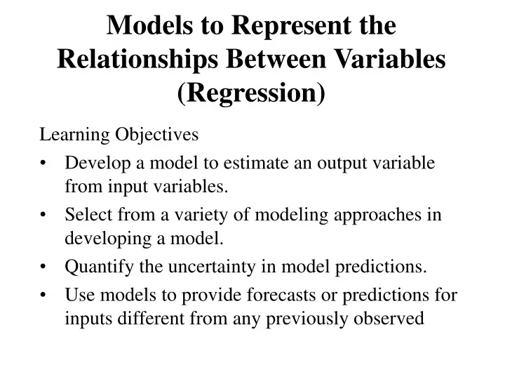
1. Models to Represent the Relationships Between Variables(Regression) Learning Objectives • Develop a model to estimate an output variable from input variables. • Select from a variety of modeling approaches in developing a model. • Quantify the uncertainty in model predictions. • Use models to provide forecasts or predictions for inputs different from any previously observed

2. Readings • Kottegoda and Rosso, Chapter 6 • Helsel and Hirsch, Chapters 9 and 11 • Hastie, Tibshirani and Friedman, Chapters 1-2 • Matlab Statistics Toolbox Users Guide, Chapter 4.

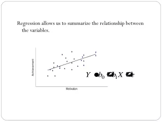
3. Regression • The use of mathematical functions to model and investigate the dependence of one variable, say Y, called the response variable, on one or more other observed variables, say X, knows as the explanatory variables • Not search for cause and effect relationship without prior knowledge • Iterative process • Formulate • Fit • Evaluate • Validate

4. Explanatory variable Independent variable x-value Predictor Input Regressor Response variable Dependent variable y-value Predictand Output A Rose by any other name...

5. The modeling process • Data gathering and exploratory data analysis • Conceptual model development (hypothesis formulation) • Applying various forms of models to see which relationships work and which do not. • parameter estimation • diagnostic testing • interpretation of results

6. Conceptual model of system to guide analysis Natural Climate states: ENSO, PDO, NAO, … Other climate variables: temperature, humidity … Rainfall Management Groundwater pumping Surface water withdrawals Groundwater Level Surface water releases from storage Streamflow

7. GSL Level Volume Area Conceptual Model Solar Radiation Precipitation Air Humidity Air Temp. Mountain Snowpack Evaporation Soil Moisture And Groundwater Salinity Streamflow

8. LOWESS (R defaults) Bear River Basin Macro-Hydrology Streamflow response to basin and annual average forcing. Runoff ratio = 0.18 Streamflow Q/A mm Runoff ratio = 0.10 Temperature C Precipitation mm

9. LOWESS (R defaults) Annual Evaporation Loss E/A Salinity decreases as volume increases. E increases as salinity decreases. E/A m Area m2

10. LOWESS (R defaults) Evaporation vs Salinity Salinity estimated from total load and volume related to decrease in E/A with decrease in lake volume and increase in C E/A m C = 3.5 x 1012 kg/(Volume) g/l

11. LOWESS (R defaults) Evaporation vs Temperature (Annual) E/A m Degrees C

12. GSL Level Volume Area Conclusions Solar Radiation Precipitation Air Humidity Air Temp. Increases Reduces Mountain Snowpack Evaporation Area Control Supplies Reduces Soil Moisture And Groundwater Contributes CL/V Salinity Dominant Streamflow

13. Considerations in Model Selection • Choice of complexity in functional relationship • Theoretically infinite choice of type of functional relationship • Classes of functional relationships • Interplay between bias, variance and model complexity • Generality/Transferability • prediction capability on independent test data.

14. Model Selection Choices ExampleComplexity, Generality, Transferability

15. Interpolation

16. Functional Fit

17. How do we quantify the fit to the data? Y ei = f(xi) - yi RSS > 0 RSS = 0 xi X X Residual (ei): Difference between fit (f(xi)) and observed (yi) Residual Sum of Squared Error (RSS) :

18. Interpolation or function fitting? Which has the smallest fitting error? Is this a valid measure? Each is useful for its own purpose. Selection may hinge on considerations out of the data, such as the nature and purpose of the model and understanding of the process it represents.

19. Another Example

20. Interpolation

21. Functional Fit - Linear

22. Which is better? Is a linear approximation appropriate?

23. The actual functional relationship (random noise added to cyclical function)

24. Another example of two approaches to prediction • Linear model fit by least squares • Nearest neighbor

25. General function fitting

26. x1 x2 x3 y x1 x2 x3 y ……… x1 x2 x3 y x1 x2 x3 y Input Output General function fitting – Independent data samples Independent data vectors Example linear regression y=a x + b + 

27. Statistical decision theory inputs, p dimensional, real valued real valued output variable Joint distribution Pr(X,Y) Seek a function f(X) for predicting Y given X. Loss function to penalize errors in prediction e.g. L(Y, f(X))=(Y-f(X))2 square error L(Y, f(X))=|Y-f(X)| absolute error

28. Criterion for choosing f Minimize expected loss e.g. E[L] = E[(Y-f(X))2]  f(x) = E[Y|X=x] The conditional expectation, known as the regression function This is the best prediction of Y at any point X=x when best is measured by average square error.

29. Basis for nearest neighbor method • Expectation approximated by averaging over sample data • Conditioning at a point relaxed to conditioning on some region close to the target point

30. Basis for linear regression • Model based. Assumes a model, f(x) = a + b x • Plug f(X) in to expected loss E[L] = E[(Y-a-bX)2] • Solve for a, b that minimize this theoretically • Did not condition on X, rather used (assumed) knowledge of the functional relationship to pool over values of X.

31. Comparison of assumptions • Linear model fit by least squares assumes f(x) is well approximated by a global linear function • k nearest neighbor assumes f(x) is well approximated by a locally constant function

32. Mean((y- )2) = 0.0459 Mean((f(x)- )2) = 0.00605

33. Mean((y- )2) = 0.0408 Mean((f(x)- )2) = 0.00262 k=20

35. Mean((y- )2) = 0.0661 Mean((f(x)- )2) = 0.0221 k=60

36. 50 sets of samples generated For each calculated at specific xo values for linear fit and knn fit MSE = Variance + Bias2

37. Dashed lines from linear regression

38. Dashed lines from linear regression

39. Simple Linear Regression Model Kottegoda and Rosso page 343

40. Regression is performed to • learn something about the relationship between variables • remove a portion of the variation in one variable (a portion that may not be of interest) in order to gain a better understanding of some other, more interesting, portion • estimate or predict values of one variable based on knowledge of another variable Helsel and Hirsch page 222

41. Regression Assumptions Helsel and Hirsch page 225

42. Regression Diagnostics- Residuals Kottegoda and Rosso page 350

43. Regression Diagnostics- Antecedent Residual Kottegoda and Rosso page 350

44. Regression Diagnostics- Test residuals for normality Kottegoda and Rosso page 351

45. Regression Diagnostics- Residual versus explanatory variable Kottegoda and Rosso page 351

46. Regression Diagnostics- Residual versus predicted response variable Helsel and Hirsch page 232

47. Regression Diagnostics- Residual versus predicted response variable Helsel and Hirsch page 232

48. QQ-plot for Log-Transformed Flows QQ-plot for Raw Flows Quantile-Quantile Plots Need transformation to Normalize the data

49. Down,  <1 (log x, 1/x, , etc.) Bulging Rule For Transformations Up,  >1 (x2, etc.) Helsel and Hirsch page 229

50. Box-Cox Transformation z = (x -1)/ ;  0 z = ln(x);  = 0 Kottegoda and Rosso page 381