Download
1 / 18
180 likes | 251 Views
Statistics 111 - Lecture 17. Testing Relationships between Variables. Administrative Notes. Administrative Notes. Homework 5 due tomorrow Lecture on Wednesday will be review of entire course. Final Exam. Thursday from 10:40-12:10 It’ll be right here in this room

E N D
Statistics 111 - Lecture 17 Testing Relationships between Variables Lecture 17 - Regression Testing
Administrative Notes Administrative Notes • Homework 5 due tomorrow • Lecture on Wednesday will be review of entire course Lecture 17 - Regression Testing
Final Exam • Thursday from 10:40-12:10 • It’ll be right here in this room • Calculators are definitely needed! • Single 8.5 x 11 cheat sheet (two-sided) allowed • I’ve put a sample final on the course website Lecture 17 - Regression Testing
Outline • Review of Regression coefficients • Hypothesis Tests • Confidence Intervals • Examples Lecture 17 - Regression Testing
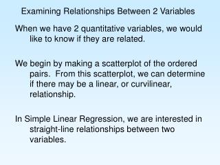
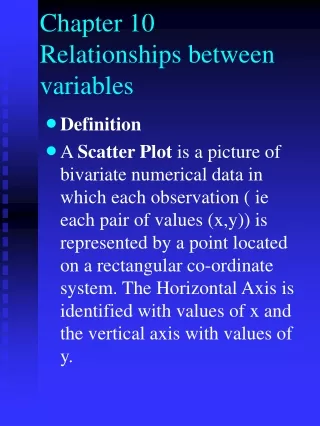
Two Continuous Variables • Visually summarize the relationship between two continuous variables with a scatterplot • Numerically, we focus on best fit line (regression) Education and Mortality Draft Order and Birthday Mortality = 1353.16 - 37.62 · Education Draft Order = 224.9 - 0.226 · Birthday Lecture 17 - Regression Testing
Best values for Regression Parameters • The best fit line has these values for the regression coefficients: • Also can estimate the average squared residual: Best estimate of slope Best estimate of intercept Stat 111 - Lecture 16 - Regression
Significance of Regression Line • Does the regression line show a significant linear relationship between the two variables? • If there is not a linear relationship, then we would expect zero correlation (r = 0) • So the slope b should also be zero • Therefore, our test for a significant relationship will focus on testing whether our slope is significantly different from zero H0 : = 0 versus Ha : 0 Lecture 17 - Regression Testing
Linear Regression • Best fit line is called Simple Linear Regression Model: • Coefficients:is the intercept and is the slope • Other common notation: 0 for intercept, 1 for slope • Our Y variable is a linear function of the X variable but we allow for error (εi) in each prediction • We approximate the error by using the residual Observed Yi Predicted Yi = + Xi Stat 111 - Lecture 16 - Regression
Test Statistic for Slope • Our test statistic for the slope is similar in form to all the test statistics we have seen so far: • The standard error of the slope SE(b) has a complicated formula that requires some matrix algebra to calculate • We will not be doing this calculation manually because the JMP software does this calculation for us! Stat 111 - Lecture 16 - Regression
Example: Education and Mortality Stat 111 - Lecture 16 - Regression
Confidence Intervals for Coefficients • JMP output also gives the information needed to make confidence intervals for slope and intercept • 100·C % confidence interval for slope : b +/- tn-2* SE(b) • The multiple t* comes from a t distribution with n-2 degrees of freedom • 100·C % confidence interval for intercept : a +/- tn-2* SE(a) • Usually, we are less interested in intercept but it might be needed in some situations Lecture 17 - Regression Testing
Confidence Intervals for Example • We have n = 60, so our multiple t* comes from a t distribution with d.f. = 58. For a 95% C.I., t* = 2.00 • 95 % confidence interval for slope : -37.6 ± 2.0*8.307 = (-54.2,-21.0) Note that this interval does not contain zero! • 95 % confidence interval for intercept : 1353± 2.0*91.42 = (1170,1536) Lecture 17 - Regression Testing
Another Example: Draft Lottery • Is the negative linear association we see between birthday and draft order statistically significant? p-value Lecture 17 - Regression Testing
Another Example: Draft Lottery • p-value < 0.0001 so we reject null hypothesis and conclude that there is a statistically significant linear relationship between birthday and draft order • Statistical evidence that the randomization was not done properly! • 95 % confidence interval for slope : -.23±1.98*.05 = (-.33,-.13) • Multiple t* = 1.98 from t distribution with n-2 = 363 d.f. • Confidence interval does not contain zero, which we expected from our hypothesis test Lecture 17 - Regression Testing
Education Example • Dataset of 78 seventh-graders: relationship between IQ and GPA • Clear positive association between IQ and grade point average Lecture 17 - Regression Testing
Education Example • Is the positive linear association we see between GPA and IQ statistically significant? p-value Lecture 17 - Regression Testing
Education Example • p-value < 0.0001 so we reject null hypothesis and conclude that there is a statistically significant positive relationship between IQ and GPA • 95 % confidence interval for slope : .101±1.99*.014 = (.073,.129) • Multiple t* = 1.99 from t distribution with n-2 = 76 d.f. • Confidence interval does not contain zero, which we expected from our hypothesis test Lecture 17 - Regression Testing
Next Class - Lecture 18 • Review of course material Lecture 17 - Regression Testing