Download
1 / 70
700 likes | 830 Views
Outline: Two variables Scatter Diagrams to display bivariate data Correlation Concept, Interpretation, Computation, Cautions Regression Model: Using a LINE to describe the relation between two variables & for prediction •Finding "the" line •Interpreting its coefficients

E N D
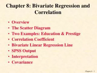
Outline: Two variables Scatter Diagrams to display bivariate data CorrelationConcept, Interpretation, Computation, Cautions Regression Model:Using a LINE to describe the relation between two variables & for prediction•Finding "the" line•Interpreting its coefficients Residuals, Prediction Errors Extensions of Simple Linear Regression Chapters 8 - 12 Unit 5Correlation and Regression:Examining and Modeling Relationships Between Variables A.05
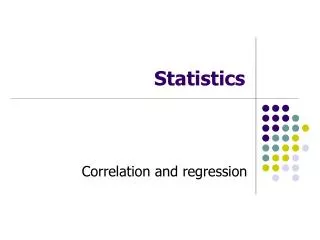
# applicants 150 10 140 cost per min. ($) 9 130 Four Scatter Diagrams 8 120 7 110 6 90 2 4 6 8 6.0 6.4 6.6 7.0 size of help wanted ad CUME rating % delinquent 45 14 last year's sales ($1000) 40 12 35 10 30 8 25 4 20 2 3 6 9 12 10 30 50 age of credit account (years) entertain. expenses (x $100)
If there is STRONG ASSOCIATION between 2 variables, then knowing one helps a lot in predicting the other. If there is WEAK ASSOCIATION between 2 variables, then information about one variable does not help much in predicting the other. Association dependent variable independent variable Usually, the INDEPENDENT variable is thought to influence the DEPENDENT variable.
1. Plot the points in a scatter diagram. 2. Find average for X and average for Y. Plot the point of averages. 3. Find SD(X), which measures horizontal spread of points, and SD(Y), which measures vertical spread of points. 4. Find the correlation coefficient (r), which measures the degree of clustering / spread of points about a line (the SD line). Summarizing the RelationshipBetween Two Variables Y Y X X
50 Wood Products Shipments and Employment, by state, 1989, excl. California 40 Employment x 100 30 20 10 0 0 50 100 150 200 250 Shipments ($ million)
469.8 7,900 246.4 4,400 205.4 2,800 186.5 3,600 175.8 3,800 142.9 2,100 139.7 2,400 120.6 1,900 118.0 1,500 104.3 1,500 89.9 1,600 73.5 1,500 72.6 1,400 71.4 1,200 53.9 800 52.4 1,400 50.1 1,200 48.1 1,400 47.0 1,100 36.7 800 27.4 500 27.3 400 22.9 300 ShipmentsEmployment Shipments ($ million) Wood Products Data
Wood Products Shipments and Employment, by state, 1989, excl. California 50 40 30 Employment x 100 20 10 0 0 50 100 150 200 250 Shipments ($ million)
The correlation coefficient measures the LINEAR relationship between TWO variables. It is a measure of LINEAR association or clustering around a line. r near +1 r near -1 r positive, r negative near 0 near 0 r =1 r = -1 Linear Association
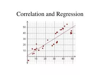
The closer the correlation coefficient is to 1 (or -1), the more tightly clustered the points are around a line (the SD line). The SD line passes through all points which are an equal # of SD's away from the average for both variables. Interpretation of r positive association negative association
Look in your textbook, pages 127 and 129. Twelve Plots, with r
Convert each variable to standard units. The average of the products gives the correlation coefficient. r = average of (z-score for X) (z-score for Y) Computing the Correlation Coefficient, r
X YX-X(X-X)2Y-Y(Y-Y)2z-score for Xz-score for Yproduct Example: Computation of r
Some Cases When the Correlation Coefficient, r, Does Not Give A Good Indication of Clustering 800 10 700 8 600 500 6 400 Y 4 300 200 2 100 0 0 0 10 20 30 40 2 4 6 8 10 0 INDEP X r = .155 r = .536
6000 5000 4000 BRAIN WEIGHT IN KG 3000 2000 1000 0 0 1000 2000 3000 4000 5000 6000 7000 BODY WEIGHT IN KG r = .933 (36 data values)
“No Elephants” 1500 1000 brain weight in grams 500 0 0 100 200 300 400 500 600 body weight in kg r = .596 (r = .887, excluding dinosaurs, elephants, humans)
all brain data,log transformed 10 5 log (brain weight) 0 -5 -10 0 10 20 log (body weight) r=.856 (all data)
120 110 P R I 100 C E 90 80 0 5 10 15 COUPON r = .883 (all data) r = .984 (without flower bonds) (Siegel)
1. Descriptive Example: Height versus Weight 2. Causal Example: Total Cost vs. Volume of Production 3. Nonsense Example: Polio Incidence vs. Soft Drink Sales Interpretation of Empirical Association
1. What is the best prediction of the dependent variable? What if the value of the independent variable is available? 2. What is the likely size of the prediction error? Fundamental Principle of Prediction 1. Use the mean of the relevant group. 2. SD of the group gives the "likely size of error." Prediction Using Correlation
Demand for LINES versus Proposed MONTHLY charge per line ($) Diamond State Telephone Company 250 200 LINES 150 100 10 15 20 25 30 35 MONTHLY
Look At The Vertical StripCorresponding to the Given X Value Y X
Graph of Averages 250 200 x x LINES x 150 x x 100 10 15 20 25 30 35 MONTHLY estimated LINES = 237.495 - 3.867 MONTHLY
The REGRESSION LINE is to a scatter diagram as the AVERAGE is to a list of numbers. The regression line estimates the average values for the dependent variable, Y, corresponding to each value, x, of the independent variable. Linearly Related Variables
If we have 2 variables, linearly related to one another, then knowing the value of one variable (for a particular individual) can help to estimate / predict the value of the other variable. • If we know nothing re. the value of the independent variable (X), then we estimate the value of the dependent variable to be the OVERALL AVERAGE of the dependent variable (Y). • If we know that the independent variable (X) has a particular value for a given individual, then we can take a "more educated guess" at the value of the dependent variable (Y). Linearly Related Variables
The REGRESSION LINE for modeling the relation between X (independent variable) and Y (dependent variable) passes through the POINT OF AVERAGES and has slope That is, associated with each increase of one SD in X, there is an increase of r SD’s in Y, on the average. The SD LINE for modeling the relation between X (independent variable) and Y (dependent variable) passes through the POINT OF AVERAGES and has slope Regression and SD Lines
The REGRESSION LINE for modeling the relation between X (independent variable) and Y (dependent variable) is also known as The REGRESSION LINE for predicting Y from X, and has the form Y = a + b x = intercept + slope x. Here, b = slope = r SD(Y)/ SD(X) a = intercept = avg(Y) - b avg(X) = avg(Y) - r [SD(Y)/ SD(X)] avg(X) Estimating the Intercept andSlope of the Regression Line
Predicted value of Y corresponding to a given value of X is Prediction from aRegression Model
TOTAL OBSERVATIONS: 21 LINES MONTHLY N OF CASES 21 21 MINIMUM 105.000 10.320 MAXIMUM 201.000 34.000 MEAN 154.048 21.581 VARIANCE 1122.648 69.623 STANDARD DEV 33.506 8.344 PEARSON CORRELATION MATRIX LINES MONTHLY LINES 1.000 MONTHLY -0.963 1.000 NUMBER OF OBSERVATIONS: 21
In the Diamond State Telephone Company example, avg (LINES) = 154.048 SD (LINES) = 33.506 avg (MONTHLY) = 21.581 SD (MONTHLY) = 8.344 r = -0.963 What are the coordinates for the point of averages? What is the slope of the regression line? Suppose the MONTHLY charge was set at $25.00. What would you estimate to be the demand for # LINES from the 62 new businesses? Suppose the MONTHLY charge was set at $15.00. What would you estimate to be the demand for # LINES from the 62 new businesses? Diamond State Questions
Suppose the MONTHLY charge was set at $50.00. What would you estimate to be the demand for # LINES from the 62 new businesses? Another Diamond State Question
Regression DEP VAR: LINES N: 21 MULTIPLE R: 0.963 SQUARED MULTIPLE R: 0.927 ADJ SQRD MULTIPLE R: 0.923 STANDARD ERROR OF ESTIMATE: 9.273 VARIABLE COEFF STD ERROR STD COEF TOLERANCE T P(2 TAIL) CONSTANT 237.495 5.732 0.000 . 41.432 0.000 MONTHLY -3.867 0.249 -0.963 1.000 -15.560 0.000 ANALYSIS OF VARIANCE SOURCE SUM-OF-SQUARES DF MEAN-SQUARE F-RATIO P REGRESSION 20819.092 1 20819.092 242.103 0.000 RESIDUAL 1633.860 19 85.993 ------------------------------------------------------------------------------------------------------------------ Regression Computer Output
1. X = Educational expenditure Y = Test scores 2. X = Height of a person Y = Weight of the person 3. X = # Service years of an automobile Y = Operating cost per year 4. X = Total weight of mail bags Y = # Mail orders 5. X = Price of product Y = Unit sales 6. X = Volume Y = Total cost of production 7. X = Calories in a candy bar Y = Grams of fat in the candy bar 8. X = Baseball slugging percentage Y = Player salary 9. X = Weight of a diamond Y = Price of the diamond 10. 11. 12. Other Examples
TOTAL OBSERVATIONS: 23 SHIPMENT EMPLOY N OF CASES 23 23 MINIMUM 22.900 3.000 MAXIMUM 469.800 79.000 MEAN 112.287 19.783 VARIANCE 9931.683 281.087 STANDARD DEV 99.658 16.766 Pearson Correlation Matrix SHIPMENT EMPLOY SHIPMENT 1.00 EMPLOY 0.979 1.00 Number of Observations: 23 Wood Products
DEP VAR: SHIPMENT N: 23 MULT R: 0.979 SQRD MULT R: 0.958 ADJ SQRD MULTIPLE R: 0.956 STD ERROR OF ESTIMATE: 21.018 VARIABLE COEFF STD ERROR STD COEF TOLER T P(2 TAIL) CONSTANT -2.781 6.868 0.000 . -0.405 0.690 EMPLOY 5.817 0.267 0.979 1.000 21.763 0.000 ANALYSIS OF VARIANCE SOURCE SUM-OF-SQUARES DF MEAN-SQUARE F-RATIO P REGRESSION .209220.316 1 209220.31 473.619 0.000 RESIDUAL 9276.710 21 441.748 ------------------------------------------------------------------------------------------- Computer Output - 1
DEP VAR: EMPLOY N: 23 MULT R: 0.979 SQRD MULT R: 0.958 ADJ SQRD MULT R: 0.956 STD ERROR OF ESTIMATE: 3.536 VARIABLE COEFF STD ERROR STD COEF TOLER T P(2 TAIL) CONSTANT 1.298 1.125 0.000 . 1.154 0.262 SHIPMENT 0.165 0.008 0.979 1.000 21.763 0.000 ANALYSIS OF VARIANCE SOURCE SUM-OF-SQUARES DF MEAN-SQUARE F-RATIO P REGRESSION 5921.363 1 5921.363 473.619 0.000 RESIDUAL 262.550 21 12.502 -------------------------------------------------------------------------------------------- Computer Output - 2
For cases with income less than or equal to $15,000, avg (Voluntary) = 6.376 SD (Voluntary) = 3.959 avg (Income) = $10,332.756 SD (Income) = $2,109.819 r = 0.896 Derive the equation for the regression line. According to this linear model, what is the estimated value for "Voluntary" in a ZIP code area with Income $12,000? ... with Income $9,500? Chicago Insurance, cont.
In virtually all test-retest situations, the bottom group on the first test will, on average, show some improvement on the 2nd test, and the top group will, on average, fall back. This is called the REGRESSION EFFECT. The REGRESSION FALLACY is thinking that the regression effect must be due to something important, not just the spread of points around theline. Regression Effect