Download
1 / 12
120 likes | 337 Views
Supply. 3 stages of production Produce in Stage II. II. III. Output. I. TPP. X. input. Output. 1. MPP. APP. X. input. 1. $/Output. y*. TVP = TPP * Py. *. X. input. $. X. 1. 1. MVP = P MPP. y. X1. MFC. X1. *. X. X. input. 1. 1. Supply.

E N D
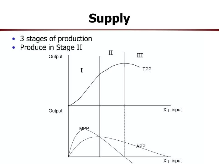
Supply • 3 stages of production • Produce in Stage II II III Output I TPP X input Output 1 MPP APP X input 1
$/Output y* TVP = TPP * Py * X input $ X 1 1 MVP = P MPP y X1 MFC X1 * X X input 1 1 Supply • 3 stages of production • Multiply MPP and APP by Price of the output
Supply • Where the supply curve comes from • Marginal cost curve MC = Px / MPPx • Average variable cost AVC = Px / APPx $ MC AVC Q/yr
Supply • Supply curve is the MC above the AVC for each firm • Supply is a schedule of quantities of output that will be offered for sale at alternative prices • Shutdown price $ MC AVC Q/yr
Supply $ $ $ $ $ $ S • Firm Supply and Industry Supply Firm 1 QY Industry QY Firm 2 QY • Factors change Industry Supply for Output Y • Technology • Costs of inputs to produce Y • Ag. Policy S0 S1 S2 P QtY
Supply • Factors that change Supply Function for firm • Price of Input • Productivity of X to produce Quantity of Y • Increased productivity Shifts MC to right • Analyze impacts on supply for the industry by starting with the firm $ MC1 MC2 AVC1 AVC2 Q/yr
Supply • New Technology – BST PST Roundup Ready crops • Increase TPP >> Higher MPP >> Lower MC • Supply shifts to the right Y TPP1 Y TPP0 MPP1 X X MPP0 $ MC0 AVC0 S0 $ S1 MC1 AVC1 Q Y /yr Q Y /yr The Industry The Firm
Supply S1 • Inflation in Input Prices and Supply Price input increases Px MC = Px / MPPx AVC = Px / APPx S0 $ Q/yr $ MC2 MC1 AVC2 AVC1 Q/yr
Supply • Cross elasticity of supply • Elasticity with respect to the price of another crop Es(QY, PX) = %ΔQY / %ΔPX Es(QY, Px) = -0.15 PX 2.5 S of Y wrt PX 2.25 ? 2,600 QY
Supply and Demand • Equilibrium price is where Demand equals Supply S1 $ S2 P 1 P 2 D q Q/yr q 2 1
Supply and Demand • Equilibrium price is where Demand equals Supply • After the crop has been harvested the supply becomes perfectly inelastic • Supply in the marketing year is S1 or S2 S1 S2 $ P 1 P 2 D q Q/yr q 2 1
Supply • Elasticity of Supply • Generally mean the elasticity of quantity supplied with respect (wrt) own price Es = %ΔQtY / %ΔPY Es = +0.20 Qt Supplied Y = Old Qt Y * [1+ Es * %ΔPy] Qt Supplied Y = Old Qt Y * [1+ Es * (Price Ynew /Price Yold) / Price Yold)] PY S 2.5 2 2,600 ? QtY