Download
1 / 137
1.48k likes | 2.03k Views
FDL’04 Tutorial September 16, 2004. Analog and Mixed-Signal System Design with SystemC. Outline. Introduction Part 1: Design and modeling issues for complex heterogeneous systems What is a complex heterogeneous system, application fields, motivations Modeling strategies for AMS systems

E N D
FDL’04 TutorialSeptember 16, 2004 Analog and Mixed-Signal System Designwith SystemC
Outline • Introduction • Part 1: Design and modeling issues for complex heterogeneous systems • What is a complex heterogeneous system, application fields, motivations • Modeling strategies for AMS systems • Part 2: Using SystemC for AMS systems • Introduction to SystemC 2.0 & use for AMS systems • Proposed AMS extensions • Part 3: Application examples • Electronic example: PLL • Automotive example: PWM driver • Telecommunication example: xDSL • Conclusions
Introduction: Tutorial Objectives • To review design and modeling issues for complex heterogeneous systems • To present a prototype implementation of modeling and simulation of mixed discrete/continuous systems in SystemC • To provide some typical application examples
Emerging Application fields (1/2) Part 1 • Ambient Intelligence Systems: • Hardware (IPs, Cores) • Software (Megabytes!) • Analog components: • Converters, PLL, … • Sensors • RF/Wireless • Automotive Systems 20XX: • Hardware (IPs, Cores) • Software (Megabytes!) • Converters, Sensors • Power electronics • Mechanical components • Maybe RF/Wireless • High Reliability+Safety!
Emerging Application fields (2/2) Part 1 • Design of future applicationshas to consider interactions between: • Digital Hardware • Analog Components • Software • Complex heterogeneous systems are superset of A/D/S + environment • Co-simulation with physicalenvironment: • Virtual prototypingreplaces “breadboards” • Virtual testbenches complement “synthetic” testbench Hydraulics Mechanics … Digital HW AnalogHW Software Realtime OS
Mixed Discrete/Continuous Systems Part 1 • Mixed Discrete/Continuous (MDC) systems exhibit a mix of: • Discrete-event or discrete-time behaviors • Continuous-time behaviors • Compared with Analog and Mixed-Signal (AMS) systems: • MDC are often far more complex:Converters, PLL, etc. are rather small components of an MDC • Coupling A/D can be modeled in a more simple, and thereby more efficient way, e.g. in discrete time steps • MDC can be more abstract, and also embrace a large fraction of software
HDL Use Part 1 • Can we use HDLs for modeling, design and verification of complex, heterogeneous systems? • Radio Eriwan‘s answer is: Yes, but … …Modeling megabytes of software in VHDL/Verilog,or integration thereof using CLI might not be very comfortable …Simulation performance would be orders of magnitudes too slow(Grimm et al. @ FDL’01: Virtual Test-Drive of Anti-Lock brake systemwould take YEARS)
HDL Use Part 1 • Can we use HDLs for modeling, design and verification of complex, heterogeneous systems? • A more helpful answer is: Yes, but … …Modeling megabytes of software in VHDL/Verilog,or integration thereof using CLI might not be very comfortable … Use SystemC for modeling hardware/software systems …Simulation performance would be orders of magnitudes too slow(Grimm et al. @ FDL’01: Virtual Test-Drive of Anti-Lock brake systemwould take YEARS) … Use abstract, behavioral models... Use application + abstraction specific means for simulationand coupling of simulators
DF model:Synchronisation implicit, static scheduling. How Can a Modeling Language Help? Part 1 • With appropriate properties we can more easily specify models, and analyze properties of a model while ignoring many implementation issues • The use appropriate modeling properties is the key to: • Abstract modeling • Efficient simulation DE model:We need explicit synchronisation, events.
Model of Computation Part 1 DefinitionA model of computation defines a set of rules that govern the interactions between model elements, and thereby specify the semantics of a model Remarks: • A model of computation can also be seen as a formal, abstract definition of a machine that executes a class of models (executable model) • A model of computation is independent from a graphical or textual language, which specifies the syntactical composition of model elements
Application + Abstraction Specific Means Part 1 • Whether a model of computation is appropriate for a modeling issue depends on: • Application, e.g.:Control systems time domain, nonlinear, asynchronous behaviorRF systems linear, static non-linearities, constant time steps • Implementation, e.g.: Analog: netlist, Digital: DE, Software: UML • Level of abstraction, e.g.: Digital: Transactions, Register transfer, Netlist, … • Modeling of heterogeneous systems at different levels of abstraction requires the use and combination of different modeling platforms
Model Facets Part 1 • Interface: • I/O ports, communication protocols, parameters • Behavior: • I/O relationships, algorithms, data flows, processes, states, equations, hierarchy • Structure: • Topological organization, connectivity, hierarchy • Geometry: • Shapes, dimensions, part assemblies • Properties: • timings, power consumption • Operating conditions: • Temperature, pressure, noise, mechanical stress, …
t t t Abstraction Part 1
MoCs for mixed continuous/discrete systems Part 1 • Continuous-Time Signal-Flow MoC: • Requirements engineering, executable specifications • Example: Simulink block diagrams • Timed Synchronous (Multirate) Dataflow MoC: • DSP algorithms • Examples: SPW (Coware), System Studio (Synopsys) • Discrete Event MoC: • Digital realization at different levels of abstraction • Example: SystemC • Continuous-Time Conservative MoC: • Analog circuits • Example: SPICE
Dataflow MoC Part 1 • Based on Process Networks • Networks of concurrent processes (actors), or actors, communicating through unidirectional unbounded FIFO channels (arcs) • Tokens represent data as atomic and usually uninterpreted elements • Processes map input tokens onto output tokens • A process fires (resumes) when enough tokens are available at its input: • Consumes input token(s) (blocking read) • Possibly computes a new internal state • Produces output token(s) (non-blocking write) • Untimed MoC
Synchronous Dataflow MoC (1/2) Part 1 • Number of consumed/produced tokens is constant for a process • Static scheduling of processes • Complete cycle: processes may be fired a finite number of times before returning to original state • Single-rate (or homogeneous) SDF • Tokens are consumed/produced one at a time (ex.: adders, multipliers) • Multi-rate SDF • Tokens are consumed/produced at various rates (ex.: decimators, interpolators, block (de)coders)
Synchronous Dataflow MoC (2/2) Part 1 • Useful for modeling digital signal processing systems • Ideal DSP behavior • Tokens = data samples • Sampling rates are rationally related • Step size between samples implicitly related to some global clock • EDA tools: • Ptolemy II (Univ. Berkeley) • SPW (Coware) • System Studio (Synopsys) • Languages: • LUSTRE, SIGNAL • Esterel • SystemC
Timed Synchronous Dataflow MoC Part 1 • Cosimulation between DSP, analog and RF domains • Common representation of signals (arcs): • Frequency info:carrier frequency fc • Time (baseband) info:in-phase component I(t), quadrature componentQ(t), t • Added attributes: • One time step and frequency carrier attached to each arc • Processes fired at constant rate • Optional I/O impedances • Time steps and freq. carriers for each arc are computed by propagation algorithms • EDA tool: Agilent Ptolemy J.L. Pino, K. Kalbasi,Cosimulating Synchronous DSP Applications with Analog RF Circuits,Proc. IEEE Asilomar Conference on Signals, Systems, and Computers,Pacific Grove, CA, Nov. 1998.
Discrete Event MoC Part 1 • Also based on process networks, but with a different communication mechanism: • Sequence of events in time • Time: integer multiple of some base time or real time • Event: (time stamp, value) • Data: tokens, enumerated symbols, logical values, numerical values • Dynamic scheduling of processes • Causality and determism ensured through delta delay iterations or throughextraction of data dependencies • Main application: Concurrent hardware systems • EDA tools: • Ptolemy II (Univ. Berkeley) • SystemC tools • VHDL(-AMS)/Verilog(-AMS)/SystemVerilog tools
Continuous-time MoC Part 1 • Based on Ordinary Differential Equations (ODEs) or Differential Algebraic Equations (DAEs) • Signals are analytical functions of time • Piecewise differentiable segments • Real valued time • Many methods to set up and to solve the system of equations: • Equation formulation methods (Nodal, Modified Nodal, Tableau, etc.) • Numerical methods (num. integration, NR linearization, linear sys. solver) • Symbolic methods • EDA tools: • Ptolemy II (Univ. Berkeley) • Matlab/Simulink (MathWorks) • SPICE variants • VHDL-AMS/Verilog-AMS tools • Applications: • Analog electrical systems • Physical systems (e.g. mechanical) • RF/microwave • Control systems
CT MoC: Signal-Flow/Block Diagrams Part 1 • Most abstract representation of physical/analog behavior • Non conservative behavior • A SF model represents a computational structure as a directed graph • Arcs are transfer functions between CT signals (nodes) • Differential relations are expressed as their equivalent discrete formulation • Block diagrams are dual representations of single port SF graphs • SFG (resp. BD) path => BD (resp. SFG) node
CT MoC: Conservative Models Part 1 • More detailed representation of physical/analog behavior • A conservative model represents the topology of the modeled system • Electrical systems: Kirchhoff’s networks meeting Kirchhoff’s laws (KCL, KVL) • Other physical systems: Generalized versions of KN and KCL/KVL laws • Bond graphs • Netlist based models: • Topological connectionof primitive elements • Elements defined byconstitutive equations • Two characteristicquantities: • Across (effort, e.g. voltage) • Through (flow, e.g. current)
CT MoC: Macromodels Part 1 • Simplified equivalent circuit or simplified system of equations that represents the I/O behavior • Goal is to achieve fast simulationwhile keeping an acceptable level of accuracy • Macromodel development techniques: • Circuit simplification • Remove circuit elements, use simpler models • Circuit build-up • Use ideal primitive elements • Progressively add non-ideal behavior • Symbolic manipulations of circuit equations
Mixing Different MoCs Part 1 • Objective is to deal with system heterogeneity • Hybrid MoC: Composition of control (FSM) and CT • Mixed-signal or mixed discrete/continuous MoC: Composition of DE and CT • MoCs are usually combined using a hierarchical approach • Interaction semanticsdefine how semantic propertiesof interacting MoCs arerelated to each other • Time is the most critical interacting property • Untimed DF and timed DE • Timed DE and timed CT
(S)DF in DE Part 1 • DF subsystems appear as zero-delay blocks • Each activation of a DF blockmust perform a complete cycle • DF subsystem may beover-constrained: • Can only fire when all ofits inputs have an event • Alternative: generate the needed data using the most recently updated value • Multi-rate SDF block: • A single event at inputs may not be enough to activate the whole block • More than one token may be produced at the output (time stamp?) W.-T. Chang, S. Ha, E.A. Lee,Heterogeneous Simulation – Mixing Discrete-Event Models with Dataflow,Journal of VLSI Signal Processing 15, pp. 127-144,Kluwer Academic Publishers, 1997.
DE and CT Part 1 • Example: VHDL-AMS initialization and time-domain simulation cycle • MoCs interact as peers (no hierarchy)
Part 2: Using SystemC for AMS Systems • Overview of SystemC 2.0 • Why C based design? • SystemC approach and use flow • Simple examples using the core language • Modeling AMS systems with SystemC 2.0 • Discrete-event modeling of continuous-time behaviors • Representation of linear dynamic systems • Adaptative time step approach • Proposed SystemC AMS extensions • Architecture of the extensions • Language constructs, class definitions
Why C based design? (1/2) Part 2 • Co-design of hardware/software systems • C/C++/UML provide means for modeling software • HDLs provide means for modeling hardware Software development Hardware development Re-partitioningrequires translation C, C++, UML,… SystemVerilog,VHDL, Verilog Systemdesign SW developers needC/C++ models
Why C based design? (2/2) Part 2 • Pragmatic approach: Use C/C++/UML for HW/SW system design Software development Hardware development C, C++, UML,… C, C++, UML, …+ means for modeling timing, concurrency and signal types SystemVerilog,VHDL, Verilog Systemdesign
The SystemC Approach Part 2 • SystemC is C++ plus a class library to support system-level HW modeling
SystemC Use Flow Part 2
Architecture of a SystemC 2.0 Model Part 2 • Separation of behavior and communication • Communication refinement: Channel's behavior may change from very abstract (e.g. transactions, protocol) to very detailed (e.g. hardware signals) without requiring to change module's behaviors
SystemC Core Language: Modules and Ports Part 2 • Structural units are called modules • Modules are inheritedfrom the class sc_module • Macro SC_MODULEdoes the job for you • Modules communicate withenvironment via ports • Ports are instances of the classes (where T denotes a data type): • sc_in<T> or sc_out<T> or sc_inout<T> • Ports are declared in the general form sc_port<class IF, int N=1> • IF = interface (see later) SC_MODULE(my_module){sc_in<type>input;sc_out<type>output;// C++ methods here (behavior) SC_CTOR(my_module){ // C++ code here (initalization) }};
SystemC Core Language: Processes Part 2 • Behavior of modules is described by discrete processes • Processes are defined as C++ methods that must be registered to the simulation kernel by the following macros: • SC_THREAD(method_name) • SC_METHOD(method_name) • Processes are activated by events which are specified in a sensitivity list following registration of the process: • sensitive[_pos|_neg] (<< [signal|event])*; #include "systemc.h"SC_MODULE(adder){ sc_in<int> in1; sc_in<int> in2; sc_out<int> outp;void do_add() { outp = in1 + in2; } SC_CTOR(adder) {SC_METHOD(do_add);sensitive << in1 << in2; }};
SystemC Core Language: Signals & FIFOs Part 2 • Modules communicate via channels • Channels are accessed via interfaces • An interface defines a set of abstractmethods that can be used for communication • Processes use interface methods read(), write(...), event(), ... • Signals are a class of primitive channels that model hardware signals • Class sc_signal<T> defines the implementations of abstract interface methods • Port sc_in<T> is derived from sc_port<sc_signal_in_if<T>,1> • FIFOs are another class of primitive channels that model bounded FIFO queues • Class sc_fifo<T> defines the implementations of abstract interface methods • Port sc_fifo_in<T> is derived from sc_port<sc_fifo_in_if<T>,1>
Hierarchical Model Example Part 2 #include "systemc.h"#include "adder.h"#include "latch.h"SC_MODULE(dut) { sc_in<bool > clk; sc_in<int > in1, in2; sc_out<int > outp; sc_signal<int> internal_signal; adder* add1; latch* latch1; … entity dut is port ( signal clk: in bit; signal in1, in2: in bit; signal outp: out bit);end entity dut;architecture str of dut is signal internal_signal: bit;begin add1: entity work.adder(dfl) port map ( in1 => in1, in2 => in2, outp => internal_signal); latch1: entity work.latch1(bhv) port map ( clk => clk; inp => internal_signal, outp => outp);end architecture str; ... SC_CTOR(dut) { add1 = new adder("add1"); add1->in1(in1); add1->in2(in2); add1->outp(internal_signal); latch1 = new latch("latch1"); latch1->clk(clk); latch1->inp(internal_signal); latch1->outp(outp); }};
Testbench Example Part 2 #include "dut.h"#include "stimuli_generator.h" int sc_main(int argc, char* argv[]) { sc_signal<int> signal1, signal2, signal3; sc_clock clock1("clock1", 1.0, SC_US); stimuli_generator stg1("stg1"); stg1.sig1(signal1); stg1.sig2(signal2); dut dut1("dut1"); dut1.inp1(signal1); dut1.inp2(signal2); dut1.out(signal3); dut1.clock(clock1); ... ... sc_trace_file *tf sc_create_vcd_trace_file("simplex"); sc_trace(tf, clock1, "clock1"); sc_trace(tf, signal1, "in1"); sc_trace(tf, signal2, "in2"); sc_trace(tf, signal3, "out"); sc_trace(tf, dut1.internal_signal, "dut_signal"); sc_start(); sc_close_vcd_trace_file(tf); return(0); }
Modeling analog modules using discrete-event SystemC • Split the equation system in non-conservative (directed) connected blocks/modules • Model the behavior of the blocks in a way that they embed his own solver • Use a SystemC-MoC to solve the overall equation system
Limitations • Modules can be connected by non-conservative signals only • No global view to the overall equation system – a non-solvable systems can’t be detected • Loops of connected modules must (should) have a delay • The system decomposition is influenced by the non-conservative signal limitation – it will not be always possible to provide general models and it can be difficult to understand the model • The modeling effort depends on the block and can be very high
Modeling analog modules with the discrete-event SystemC • Split the equation system in non-conservative (directed) connected blocks/modules • Model the behavior of the blocks in a way that they embed his own solver • Use a SystemC-MoC to solve the overall equation system
Split the equation system into non-conservative modules • Some guidelines • Model the (black box) behavior of the interested values – use your system knowledge • If possible consider an output resistance as zero and/or the following input resistance as infinite • Split the wires into directed signals which are carry the current or the voltage • Try to split into linear dynamics and non-linear static's • Split into control and signal flow
Modeling analog modules with the discrete-event SystemC Principle: • Split the equation system in non-conservative (directed) connected blocks/modules • Model the behavior of the blocks in a way that they embed his own solver • Use a SystemC-MoC to solve the overall equation system
Model the modules in a way that they embed the solver Part 2 SC_MODULE(kv2w) { sc_quantity_in v2w; sc_quantity_out vtr; //control de - inport sc_in<double> k_v2w; void sig_proc(); SC_CTOR(kv2w) { SC_THREAD(sig_proc); } }; void kv2w::sig_proc() { while(true) { double v2w_tmp=v2w.read(); double vtr_tmp; vtr_tmp=k_v2w.read() * vtr_tmp; vtr.write(vtr_tmp); } }
Modeling linear analog dynamic behavior Part 2 • Example: RC low pass SC_MODULE(low_pass) {sc_quantity_in u; sc_quantity_in y;double TAU; // time constantdouble state; // internal state void sig_proc() { sc_time DT(10, SC_US); double DDT = DT.to_seconds();while (true) { state = (state*TAU + u.read()*DDT) / (TAU + DDT); y.write(state); } } SC_CTOR(low_pass) { // initializations TAU = 2.0e-4; state = 0.0; // register thread SC_THREAD(sig_proc); } };
“Analog” Representation of linear dynamic Systems • Transfer function • Zero-Pole representation • State Space equations • Easy extraction from networks, ... • Operational amplifier, analog filters • Good state control
Bilinear Transform timediscretization Filter identification Transformation to Discrete Time (1/2) Part 2 MATLAB Code: : [bbz,abz]=bilinear(b,a,FS); : #discrete filter identification #weigthing vector wt=[1:-1/size(w,2):1/size(w,2)]; [bz,az]=invfreqz(hs,w/FS,2,2,wt,100,0.001);
difference equations, we can implement in C++, e. g. Solving of discrete Time System Representation void hz::sig_proc() {//straigthforward implementation //input shift registerfor(i=0;i<n;i++) zu[i+1]=zu[i]; zu[0]=u; //calculate nominator for(i=0,y=0.0;i<=n;i++) y+=bd[i]*z[i]; //calculate denominator for(i=1;i<=m;i++) y-=ad[i]*zy[i]; y=y/ad[0]; //y-shift register for(i=0;i<m;i++) zy[i+1]=zy[i]; zy[0]=y; } • Transfer function • State Space
Modeling conservative Blocks • Encapsulation into one block • Transformation to a non conservative system • Transform this system to a prepared system representation (transfer function, state space equations)
V I or Modeling linear electrical Networks