Download
1 / 18
200 likes | 402 Views
VSP modeling, velocity analysis, and imaging in complex structures. Yue Du With Mark Willis, Robert Stewart. May. 16th, 2013 Houston, TX. Work Outline. 1. Introduction to Vertical seismic Profile(VSP); 2. VSP modeling investigation; 3. Velocity model building and imaging.

E N D
VSP modeling, velocity analysis, and imaging in complex structures Yue Du With Mark Willis, Robert Stewart May. 16th, 2013 Houston, TX
Work Outline • 1. Introduction to Vertical seismic Profile(VSP); • 2. VSP modeling investigation; • 3. Velocity model building and imaging.
Why Vertical Seismic Profiling (VSP)? High-resolution imaging example Representation of a 3D VSP imaging survey. (Hornby et al., 2006)
Gulf of Mexico Velocity Model Coordinates: X: 0-10025 m Y: 0-10025 m Z: 0-8000 m Grid no.: 402*402*1601 Grid Spacing: 25m*25m*5m Example for a 2D plane Shots Siliciclastic series Carbonate limestone shales Carbonate Receivers Siliciclastic series Carbonate limestone (Hallliburton/Pemex)
Ray Tracing(RT) modeling results Ray Tracing(RT) model for far-offset (i.e. 13th shot) 1st. Rec. gather
Acoustic FD modeling results: 1st. Rec. gather
Comparison between FD and RT modeling SeisSpace acoustic FD modeling RT modeling
Comparison between acoustic and elastic FD modeling: Fist break Shear wave?
Imaging results comparison between SeisSpace acoustic FD modeling and RT modeling Data SeisSpace acoustic FD modeling RT modeling Receiver
Kirchhoff Migration results: 5% fast velocity_v/0.95 Kirchhoff Migration results: 20% fast velocity_v/0.8 Kirchhoff Migration results: 20% slow velocity_v/1.2 Kirchhoff Migration results: 5% slow velocity_v/1.05 Kirchhoff Migration results: correct velocity_v
Geometry for Migration in a CIG gather 0 Setting tsig to tsg can get migration in a CIG(bb) bb s 0 z g For this shot and receiver pair, the arrival time of the actual reflection (LHS of equation), will have to match the “migration time” where it is put in the migrated image (RHS of equation). z - g s - bb R bb Migration Equation: 2R
Methodology:Tilted Ellipse In UO’V coordinates: Intersection:
The intersections of the tilted migration ellipses Diagram showing the intersections of the tilted migration ellipses with a CIG. (a) For the migration velocity equal to the true velocity (2500m/s). (b) For a slower migration velocity (2000m/s)
Wrong Migration Velocity Pulls in the Wrong Data Numerical examples for residual moveout in a single receiver offset with a CIG (bb=-500m). (a) For the migration velocity equal to the true velocity (2500m/s). (b) For a slower migration velocity (2000m/s). The red curve is the solution to the MI equation. The extreme point will be the depth of migrated reflector.
Residual moveout after migration for a numerical example (a) Residual moveout in the migrated, unstacked trace domain, M(s, g, z). (b) The residual moveout in a migrated, stacked trace domain, M(g, z), derived from the black stationary phase points in panel a.
Residual moveout for layer 4 comparing with the migration results A (Vlayer4=0.9Vtrue) A’ (Vlayer4=0.95Vtrue) B (Vlayer4=Vtrue) C (Vlayer4=1.05Vtrue) C’ (Vlayer4=1.1Vtrue) Residual moveout for layer 4 in the multi-layer velocity model. Migration results with changing interval velocity for layer 4 in case A and C’.
Acknowledgements • Thank you for Dr. Rob Stewart and AGL friends for the support and guidance in my Ph.D. studies • Thank you for Dr. Mark Willis and colleagues at Halliburton Thank you!