Download
1 / 38
380 likes | 542 Views
Imaging complex structures in the ionosphere Cathryn Mitchell, Department of Electronic and Electrical Engineering. Outline. Introduce tomography as a concept Outline some simple algorithms A real system - Earth’s upper atmosphere (the ionosphere) Other systems and applications. ?. ?.

E N D
Imaging complex structures in the ionosphere Cathryn Mitchell, Department of Electronic and Electrical Engineering
Outline Introduce tomography as a concept Outline some simple algorithms A real system - Earth’s upper atmosphere (the ionosphere) Other systems and applications
? ? ? ? What is tomographic imaging? e.g. Take a grid containing four numbers Each number represents the magnitude of the property of the system For example the density of an object It could be the density of human body tissue X-ray absorption is proportional to density (left. Cranial blood vessels imaged by xray tomography)
? ? ? ? How does tomography work? Take measurements that pass through and are affected by an object By taking many measurements from different angles you can determine the spatial distribution of the integrated quantity For example if each of the above measurements (integrated quantities) are all equal to 10, find the density in each pixel
? 5 9 7 ? 5 3 1 1 ? 3 5 ? 5 9 7 Were there enough measurements? Four equations, four unknowns … but there are many possible answers … etc Equations not all independent
? 2 ? 8 ? 8 ? 2 If I can’t change the geometry? Need some prior information For example, if you know that the second pixel is four times the value of the first then you can solve the equations with these measurements
? ? ? ? If I can choose the geometry? (1) Formulate as a set of equations, e.g. A11x1+A12x2=10 A23x3+A24x4=10 A31x1+A33x3=10 A13x3 = 5 * 1.41 ... M1 M2 M3 M4 The influence of each measurement, M, is weighted by its length, A, through each density, x
5 5 5 5 If I can choose the geometry? (2) Put in the path lengths and the unknowns are now only the densities 1 x1+ 1 x2=10 1 x3 + 1 x4=10 1 x1+1 x3=10 1.41 x3= 5 * 1.41 ...
Questions about imaging • What is the fundamental thing that is measured? Attenuation of an x-ray? Change in a radio signal phase? How does this relate to my unknown quantity? • How accurately did I measure it? How does this error relate through to my solution? (real data can be strange) • Have I measurements over many angles? If not then how can I compensate for missing information? • Do I even know the spatial path of the integral? Is the signal refracted? Is the problem linear?
Backprojection • Set all the image pixels along the ray pointing to the sample to the same value • The final backprojected image is then taken as the mean of all the backprojected views. Diagram from http://www.dspguide.com
Iterative algorithms • All the pixels in the image array are set to some arbitrary value. • An iterative procedure is then used to gradually change the image array to correspond to the profiles. • The algorithms attempts to address: how can the pixel values intersected be changed to make them consistent with this particular measurement? • An iteration cycle consists of looping through each of the measured data points.
The Algebraic Reconstruction Technique x is the density, j is the pixel index, k is the iteration index, y is the measurement of ray index, i, and delta the path length. ART was used in the first commercial medical CT scanner
ionosphere Earth What is the ionosphere? The ionosphere can be considered to be basically a thick shell of free electrons surrounding the Earth, starting at about 90 km altitude and extending to well beyond 700 km altitude
What is the ionosphere? It is where our atmosphere meets space - starting at 100 km above the Earth The thin atmosphere is bombarded with solar radiation and becomes ionised – hence the name the ionosphere The ionisation consists of a dynamic sea of atoms or molecules and free electrons The number of free electrons in a given volume is referred to as the electron density
What is complex about it? Physics - the ionosphere is connected to the Sun (through radiation and magnetic fields) and to the Earth (through dynamical coupling to the lower atmosphere) – there are many inputs to the ionosphere system
Solar bombardment of the Earth Acknowledgements for NASA movie
What is complex about it? Physics - the ionosphere is connected to the Sun (through radiation and magnetic fields) and to the Earth (through dynamical coupling to the lower atmosphere) – there are many inputs to the ionosphere system Measurements - the ionosphere slows and refracts radio signals – hence ray bending means that some measurement paths are known and some are not. There are many measurements that give different information Structure – the electron density can form structures on many spatial scales – from metres up to thousands of kilometres. Knowledge of all of these scales is useful for different science and applications
Tomographic inversion (1) Path integrals (A) are determined through a 3-D voxel representation of the ionosphere of electron concentration (x) for TEC observations (b).
Tomographic inversion (2) A relatively short period is chosen for the time-dependent inversion, for example one hour, and data collected at typically 30 second intervals are considered. The mapping matrix, X, is used to transform the problem to one for which the unknowns are the linear changes in coefficients (X) of a set basis functions
Tomographic inversion (4) To put this into words. First we formed a set of mathematical models of the ionosphere – these were spherical harmonics and orthogonal functions Next the corresponding values along each measurements path was found by the appropriate integration through each model A least-squares fit is made between the measurements and all the corresponding paths through the models to find an appropriate weighting (W) for each model These weightings are applied back to the model electron densities
MIDAS imaging Horizontal Variation Spherical Harmonics Model (eg IRI) • Graphics options • Vertical profiles of Ne • Horizontal profiles of Ne • TEC maps • Electron concentration images (latitude vs height) at one longitude. • Electron concentration images (longitude vs height) at one latitude. • TEC movies • Electron concentration movies Inversion type 2-D (latitude-height or thin shell) 3-D (2-D with time evolution or latitude-longitude-altitude) 4-D (latitude-longitude- altitude-time) Height profile (to create EOFS) Thin Shell (variable height) Chapman profiles Epstein profiles Models (eg IRI) Co-ordinate frame Geographic Geomagnetic TIME: None Zonal/Meridional Zonal/Meridional & Radial Diagram showing options in ionospheric part of MIDAS program.
Tomographic imaging – MIDAS – northern hemisphere Acknowledgements: IGS network
Users of images of the ionosphere GPS navigators – the ionosphere induces an error on the position and sometimes a fading of GPS signals – aircraft landing systems and surveyors Radio communications planners – the ionosphere refracts lower frequency signals and can distort signals at higher frequencies Scientists – investigating the interactions between the Earth and the Sun
Research applications • The ionosphere causes two problems for GPS navigation: • Group delay to the signal propagation time that is proportional to the total electron content. This can change the apparent position by tens of metres. • Scintillations of the signal are related to small-scale irregularities in electron density. These can cause temporary loss of the signals.
Research applications These effects are not an issue for most GPS users but they are important for safety-critical applications. A clear example of a GPS signal broken up in an auroral arc has already been identified Relating the physics to the impacts on systems is important, especially in new technologies like GPS and the new European Galileo.
More examples of tomography • Oil exploration • Mapping sea temperatures • Imaging of human brain • Bone structure in race horses • Atmospheric water vapour
Other areas of tomography “From oil pipelines to pork pies, electromagnetic tomography is providing new ways to look inside industrial processes” http://physicsweb.org/articles/world/16/6/8 “oil, gas and water flowing in a pipeline from the North Sea can be imaged” “A uniform and consistent product is often essential for commercial success, and images from the inside of mixing vessels can determine when the contents are of even quality. On food production lines, for example, defects in fruit can be automatically detected”