Status and Outlook for Observation-Based Quantitative Precipitation Estimation at High Latitudes

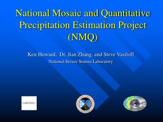
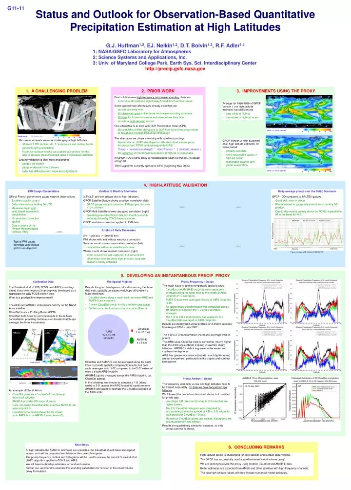
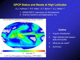
1. AMSR-E AIRS A B GPCP V.1 (mm/d) 1988-99 A CloudSat C C B A Reflectivity Low High B GPCP V.2 (mm/d) 1988-99 1. A CHALLENGING PROBLEM 2. PRIOR WORK 3. IMPROVEMENTS USING THE PROXY C Best solution uses high-frequency microwave sounding channels - try to slice atmospheric signal away from difficult surface issues. Some approximate alternatives already exist that can - provide answers now. - fill inter-swath gaps in the future microwave sounding estimates. - fill holes for future microwave estimates where they falter. - provide a multi-decadal record. One alternative is to work with OLR Precipitation Index (OPI) - Xie and Arkin (1998): deviations in OLR from local climatology relate to deviations in precip from local climatology The alternative we chose is working with satellite soundings - Susskind et al. (1997) developed a calibrated cloud volume proxy for precip from TOVS (and subsequently AIRS) Precip = revised cloud depth * cloud fraction * ƒ ( latitude, season ) - the accuracy of interannual fluctuations at high lat. is reasonable In GPCP, TOVS/AIRS proxy is recalibrated to SSM/I at mid-lat., to gauge at high lat. TOVS algorithm currently applied to AIRS (beginning May 2005) Average for 1988-1999 of GPCP Version 1 (no high-latitude estimate) had deficiencies - data voids at high lat. - low values in high-lat. ocean GPCP Version 2 (with Susskind et al. high-latitude estimate) for same period - globally complete - more-reasonable values in high-lat. ocean - reasonable balance with global evaporation Microwave etrievals are more challenging at high latitudes - different T, RH profiles; sfc. T; tropopause and melting levels - generally light precipitation - frozen/icy surface knocks out scattering channels (for this time in January most of Eurasia lacks a microwave estimate) Ground validation is also more challenging - gauges are sparse - gauge undercatch more severe - radar has difficulties with snow and bright band 4. HIGH-LATITUDE VALIDATION Daily-average precip over the Baltic Sea basin GPCP 1DD compared to BALTEX gauges - Good skill, even in winter - Bias is related to gauge adjustment from monthly SG product - Day-to-day events entirely driven by TOVS (in parallel to IR in the band 40°N-S) FMI Gauge Observations Official Finnish government gauge network observations - Excellent quality control - Daily observations ending 06 UTC - Measures liquid and solid (liquid equivalent) precipitation - No wind-loss correction applied - Data courtesy of the Finnish Meteorological Institute (FMI) Gridbox E Monthly Anomalies 2.5°x2.5° grid box (shape due to high latitudes) GPCP Satellite-Gauge shows excellent correlation (left) - GPCP gauge analysis based on FMI gauges, but only ~10% of them GPCP Multi-Satellite shows very good correlation (right) - climatological calibration to SG, but month-to-month anomaly driven by TOVS-based estimate GPCP wind-loss correction applied to FMI data Gridbox 5 Daily Timeseries 2°x1° grid box (~100x100 km) FMI shown with and without wind-loss correction Summer month shows reasonable correlation (left) - competitive with other satellite estimates Winter month shows modest correlation (right) - event occurrence well-captured, but amounts low - other winter months show high amounts; long-term scatter is nearly unbiased Precipitation (mm/d) Typical FMI gauge coverage with various grid boxes depicted Figure courtesy of B. Rudolf, DWD/GPCC 1997 February January Precip Frequency - Ocean The major issue is getting comparable spatial scales: - CloudSat and AMSR-E footprints were separately averaged along the nadir track to the length of AIRS footprints (1-D averages). - AMSR-E data were averaged directly to AIRS footprints (2-D). - An approximate transformation was computed using a 4th-degree fit between the 1-D and 2-D AMSR-E averages. - The 1-D to 2-D transformation was applied to the CloudSat data averaged to AIRS footprints. Results are displayed in zonal profiles for 3-month seasons from August 2006 – July 2007. The 1-D to 2-D transformation increases coverage (red vs. green). The AIRS-scale CloudSat (red) is somewhat (much) higher than the AIRS-scale AMSR-E (blue) in low/mid- (high) latitudes. AMSR-E’s deficit is greater in the winter and southern hemispheres. AIRS has greater occurrence (but with much lighter rates) almost everywhere, particularly in the tropics and summer hemisphere. AIRS 40 x 40 km (at nadir) CloudSat 1.4 x 2.5 km AMSR-E 4 x 6 km Precip Amount - Ocean The frequency work tells us low and high latitudes have to be treated separately. To date we have focused on low latitudes. We followed the procedure described above, but modified for precip rate: - Low (high) 1-D rates tend to map to 2-D rate that are higher (lower). - The 2-D CloudSat histogram was computed by accumulating the entire spread of 1-D to 2-D values for each particular CloudSat 1-D rate. - Maxed-out CloudSat values are tracked; histograms are accumulated with and without Results are qualitatively similar for seasons, so only boreal summer is shown. 13-19 July 2007 JJA 6. CONCLUDING REMARKS High-latitude precip is challenging for both satellite and surface observations. The GPCP has successfully used a satellite-based “cloud volume proxy”. We are seeking to revise the proxy using modern CloudSat and AMSR-E data. Better estimates are expected from AMSU and other satellites with high-frequency channels. The best high-latitude results will likely include numerical model estimates. G11-11 Status and Outlook for Observation-Based Quantitative Precipitation Estimation at High Latitudes G.J. Huffman1,2, EJ. Nelkin1,2, D.T. Bolvin1,2, R.F. Adler1,3 1: NASA/GSFC Laboratory for Atmospheres 2: Science Systems and Applications, Inc. 3: Univ. of Maryland College Park, Earth Sys. Sci. Interdisciplinary Center http://precip.gsfc.nasa.gov 5. DEVELOPING AN INSTANTANEOUS PRECIP PROXY Calibration Data The Susskind et al. (1997) TOVS (and AIRS) sounding-based cloud volume proxy for precip was developed as a regression on daily FGGE station data. What is a good path to improvement? The AIRS and AMSR-E instruments both fly on the NASA Aqua satellite. CloudSat hosts a Profiling Radar (CPR). CloudSat trails Aqua by just one minute in the A-Train constellation, providing continuous co-located match-ups amongst the three instruments. The Spatial Problem • Despite the good time/space co-location among the three data sets, spatially consistent matchups still present a huge challenge: • - CloudSat views along a nadir track, whereas AIRS and AMSR-E are scanners. • - Current CloudSat precip is only available over ocean. • - Furthermore, the footprint sizes are quite different: • CloudSat and AMSR-E can be averaged along the nadir track to provide spatially comparable results, but both such averages look “1-D” compared to the”2-D” extent of even a single AIRS footprint. • AMSR-E can be averaged across the AIRS footprint, but CloudSat cannot. • In the following, we choose to compute a 1-D (along-nadir) to 2-D (across the AIRS footprint) transform from AMSR-E and use it to estimate the CloudSat average at the AIRS scale. An example off South Africa: - CloudSat provides a “curtain” of cloud/precip data at all latitudes. - AMSR-E provides 2D maps of precip. - Here, sfc-based CloudSat echo matches AMSR-E rain area (at point B). - CloudSat echo based above the sfc shows up in AIRS, but not AMSR-E (near A and C). Next Steps At high latitudes the AMSR-E estimates are unreliable, but CloudSat should have few capped values, so it will be computed and taken as the correct histogram The precip frequency profiles and histograms will be used to rescale the current Susskind et al. (1997) algorithm applied to TOVS and AIRS. We still have to develop estimates for land and sea ice. Further out, we intend to examine the sounding parameters for revision of the cloud volume proxy formulation.