Validation of Coastwatch Ocean Color products

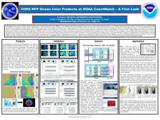
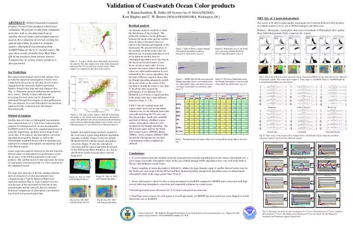
1. Validation of Coastwatch Ocean Color products S. Ramachandran, R. Sinha (SP Systems Inc @ NOAA/NESDIS) Kent Hughes and C. W. Brown (NOAA/NESDIS/ORA, Washington, DC) NRT QA of Coastwatch products The goal is to be able to make quality assessments for Coastwatch Ocean Color products in a timely manner to be of use to NOAA managers and other users. Products: Histograms, scatter plots, time series of residuals of Chlorophyll, nLw, quality flags (Individual granule, Daily composite, by region) ABSTRACT:NOAA Coastwatch routinely produce Ocean Color products which need validation. We present results from validation activities with in situ data match up of satellite derived values and residual analysis used in the evaluation of several existing bio-optical algorithms designed to estimate surface chlorophyll concentration from SeaWiFS data for the U.S. coastal waters. We also show results from the Near-Real Time QA of our products from various sensors. Comparisons of various sensor products is also presented. Residual analysis An alternate analysis would be to study the distribution of the residuals. We define the residual to be the difference between the insitu value and the satellite derived value of the pixel closest in match to the latitude and longitude of the insitu point. We present below plots of the residual versus the insitu value for different sets of ground truth data as well as for different satellite derived chlorophyll algorithms used. Any bias in the data from the ideal mean of zero shows clearly in such a plot. It even separates the region where chlorophyll values are either underestimated or over estimated by the various algorithms. For the Gulf of Mexico region it shows that the Stumpf algorithm adequately models the in-situ values as the scatter of the residuals is around the mean of zero (Fig. 5). In all the other regions the performance is not optimal. Even SEADAS oc4v4 shows a significant bias as the mean value has a slope different from zero (Figs. 6, 7, 8). Figure 5. Gulf of Mexico region Stumpf Chlorophyll algorithm residual as function of insitu (units: mg m-3) Figure 6. Balch data set for the North east coast using default SEADAS OC4v4 algorithm (units: mg m-3) Figure 1. A map of all the insitu chlorophyll data used in the analysis. The data sample used in the study adequately represents the US east and west coastal regions. More samples are required for the Great Lakes region. Sea Truth Data Bio-optical measurements used in this analysis were provided by numerous investigators. Cruises were conducted in all seasons in optically diverse waters ranging from the extremely shallow and turbid Pamlico Sound to the deep and clear Sargasso Sea (Fig. 1). Numerous agencies and programs sponsored these cruises. Details of data collection and processing for each cruise can be obtained from individual Principal Investigators or their publications. The vast majority of in-situ chlorophyll concentrations employed in this evaluation were determined fluorometrically. Fig 9. Shows the different sensor retrievals (Aqua, Terra & SeaWiFS) for the same day for two different Coastwatch regions. The scatter plots (Aqua vs. Terra, Aqua vs. SeaWiFS, Terra vs. SeaWiFS and the corresponding residuals are also shown. Figure 7 . NMFS data (North east) using the Stumpf algorithm shows overestimation for low chlorophyll values and underestimation for higher chlorophyll concentration. (units: mg m-3) Figure 8. The above Balch data using the Stumpf atmospheric correction and chlorophyll algorithm (units: mg m-3) Table 1 lists the residual mean and sigma values from various algorithms studied so far for the different insitu data sets collected along the US east coast. The Great Lakes, South east coast(SE) and Gulf of Mexico (GoMex) region surface chlorophyll values are well modeled by the Stumpf algorithm. The OC4v4 does quite well for the North East coastal waters (MWRA, Balch, NMFS). In the estuaries (EMAP, CBP) around the Chesapeake bay the land contamination makes comparisons difficult. Southeast Gulf of Mexico Westcoast Figure 2 . The large scatter makes it difficult to determine the quality of the model used in deriving the chlorophyll values. The global fit also shows insufficient discriminating power between different algorithms as the coastal waters in different regions of the CONUS have different behavior. Method of Analysis Satellite derived values of chlorophyll concentration were extracted from a 5 x 5 pixel box centered on the position of contemporaneous in-situ measurements. SeaWiFS Level L1A files were acquired and processed using the climatologic ancillary meteorological and ozone data. A bio-optical and atmospheric correction algorithm developed by Stumpf as well as the NASA/GSFC SeaWiFS Project OC4v4 algorithm was employed to estimate chlorophyll concentrations in all Coast Watch regions. Linear regression analysis between in-situ and remotely-derived values of chlorophyll was performed to assess the accuracy of the NOAA-generated ocean color products. The satellite-derived value represents the mean of valid pixels extracted from the 5 x 5 box centered on the sampling location. Sample chlorophyll image products created for the coast watch region using different algorithms currently available. Figure 3a uses the default SEADAS OC4v4 with the default atmospheric correction. Figure 3b uses the atmospheric correction and bio-optical algorithm developed by the NOS group (Rick Stumpf et. al.). Fig 4a and 4b show results from the latest versions being used. Great Lakes Carribean Extended Pacific Fig 10. Time series of the mean of the residuals above calculated for daily composite and their respective sigma is shown for the different regions Table 1. Residual mean and sigma values for four algorithms using eight in-situ data sets. • Conclusions: • It can be inferred from the residual versus the insitu plot how well the algorithm derives the surface chlorophyll over a given range of possible chlorophyll values. In the case of Rick Stumpf (NOS) algorithm it does very well in the Gulf of Mexico and Southeast coastal waters. • Sparse sampling of insitu data makes it difficult to validate the large dynamic range of satellite derived values seen for the North east coast using both the OC4v4 and Rick Stumpf algorithm, though both algorithms seem to underestimate chlorophyll values in the range greater than 10 mg m-3. • Issues with negative values for nLw is more prominent for SeaWiFS compared to MODIS and is associated with high aerosol (affecting atmospheric correction) and suspended sediments in coastal waters. • Overall agreement across all sensors for % of clear ocean pixels in each scene. • Cloud flags across sensors for each region in overall agreement, yet MODIS has more pixels per scene flagged as cloudy than in the case of SeaWiFS. The slope and intercept of the line relating remotely derived estimates to in-situ measurements was computed using a Type II, Reduced Major Axis regression analysis (Fig 2). Type I analysis was not used because of the uncertainty in both the in-situ measurements and the remotely derived estimates. Statistical comparisons of chlorophyll concentration were based on log-transformed data. Figure 3b. Day 16, 2002 with Stumpf algorithm Figure 3a. Day 16, 2002 with SEADAS OC4v4 Fig 4a. Day 189, 2005 with SEADAS OC4v4 Fig 4b. Day 189, 2005 with Stumpf algorithm Fig 11. Summary statistics on clear ocean pixel % (1st row); Cloud fraction (2nd row) ; negative nLw fraction (3rd row); Absorbing aerosol fraction (4th row) are shown for the Westcoast, Southeast and Northeast regions respectively. Acknowledgement: We thank the Principal Investigators for providing their in-situ measurements to us. Support for this project was provided by NOAA/NESDIS funding to C.W.B.