Understanding Standardization and Z-Scores in Normal Distributions
230 likes | 362 Views
This lesson explores the concept of standardizing individual values through Z-scores, which allows for comparison across different distributions. It covers the key principles of the standard normal distribution, the process of standardizing values, and how to interpret Z-scores. The example of women's heights illustrates the standardization process, while the comparison of batting averages among historic baseball players demonstrates its practical application. Additionally, exercises engage learners in using Z-tables for finding proportions related to the standard normal distribution.

Understanding Standardization and Z-Scores in Normal Distributions
E N D
Presentation Transcript
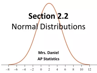
Standard Normal Calculations2.2 b cont. Target Goal: I can standardize individual values and compare them using a common scale Hw: pg 105: 13 – 15, pg 132: 54ab(see 53 as example), 55, 56, 58, 59.
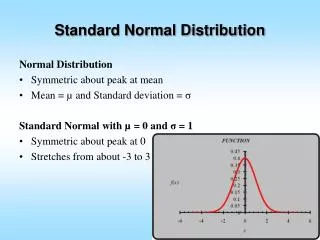
Standardizing and Z-Scores All normal curves are the same if we measure in units of size σ about the mean μ as center. Changing to these units is called standardizing. • If x is an observation from a distribution that has mean μ and standard deviation σ, then the standardized value, called the z-scoreof x is:
Standardizing and Z-Scores A z-score tells us how many standard deviationsthe original observationfalls away from the meanand inwhich direction. • Observations larger than the mean are positive. • Observations smaller than the mean are negative.
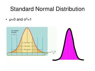
Standard Normal Distribution • If a variable x has any normal dist. N(μ,σ), • Then the new standardized variable produced has the standard normal distribution. OriginalStandardizeNew x, N(μ,σ) z z, N(0,1)
Ex 1: Standardizing Women’s Heights • The heights of young women are approx. normal with μ = 64.5 inches and σ = 2.5 inches. • The standardized height is: z = (height – )/ A women’s standardized height is the number of standarddeviations by which her height differsfrom the mean height of all young women. 64.5 2.5
μ = 64.5 inches and σ = 2.5 64.5 2.5 • A women 68 inches has a standardized height ? z = ( – )/ = standard deviations above the mean. • A women 5 feet tall has a standardized height? standard deviations below the mean. 68 1.4 z = (60 – 64.5)/2.5 = -1.8
Standardizing • Standardizing gives a common scale and produces a new variable that has the standard normal distribution.
Exercise 2: Comparing Batting Averages • Three landmarks of baseball achievement are Ty Cobb’s batting average of .420 in 1911, Ted Williams .406 in 1941, and George Brett’s .390 in 1980. • These batting averages cannot be compared directly because the distribution of major league batting averages has changed over the years. • While the mean batting average has been held roughly constant by rule changes and balance between hitting and pitching, the standard deviation has dropped over time.
Here are the facts: Decade Mean Std. Dev 1910’s .266 .0371 1940’s .267 .0326 1970’s .261 .0317 Compute the standardized batting averages for Cobb, Williams, and Brett to compare how far each stood above his peers.
Who was the best among his peers? • Cobb(.420 ); 1910’s (.266,.0371) : z = z = 4.15 • Wiliams(.406 ); 1940’s(.267,.0326): z = 4.26 • Brett(.390 ); 1970’s(.261,.0317): z = 4.07 Williams z-score is the highest. .420 - .266 .0371
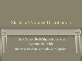
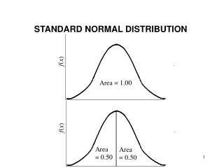
Normal Distribution Calculations • The area under a density curve is a proportion of the observations in a distribution. • After standardizing, all normal distributions are the same. • Table A gives areas under the curve for the standard normal distribution.
The table entry for each z value is the area under the curve to the left of z. • Be careful if the problem asks for the area to the left or to the right of the z value. • Always sketch the normal curve, mark the z value, and shade the area of interest.
Ex. 3 Using the Z Table • Find the proportion of observations from the standard normal distribution that are less than 1.4. • Look in Table A to verify
Ex 1. Cont. Women’s Height • What proportion of all young women are less than 68 inches tall. (We already calculated z). • The area to the left of z = 1.4 under the standard normal curve is the same as the area to the left of x = 68. (Use Table A)
Finding Normal Proportions 1. State: the problemin terms of the observed variable x. Draw a picture of the distribution and shade the area of interest under the curve. 2. Plan:Standardize x and restate the problem in terms of a standard normal variable z. Draw a picture to show the area of interest under the standard normal curve. 3. DO: Find the required area under the standard normal curve, using Table Aand the fact that the total area under the curve is 1. 4. Conclude:Write your conclusion in the context of the problem.
Exercise 4: Table A Practice • Use Table A. In each case, sketch a standard normal curve and shade the area under the curve that is the answer to the question. a. z < 2.85 b. z > 2.85 c. z > -1.66 d. -1.66 < z < 2.85 .9978 1-.9978 = .0022 1 - .0485 = .9515 .9978 -.0485 = .9493
Exercise 5: Heights of American Men The distribution of adult American men is approximately normal with mean 69 inches and standard deviation 2.5 inches. a. What percent of men are at least 6 feet (72 inches) tall? Step 1: State the problem. We want the proportion of men’s heights with x ≥ 72 inches.
Step 2: Plan 69 2.5 • mean 69, standard deviation 2.5 inches Step 2: Standardize and draw a picture. x ≥ 72 (x - μ)/σ ≥ ( - )/ z ≥ 1.2 72
z ≥ 1.2 Step 3: Do -Use the table. Area is: 1 – P( z < 1.2 ) = 1 – 0.8849 = 0.1151 Step 4: Conclude in context. About 11.5% of all adult men are at least 6 feet tall.
b. What percent of men are between 5 feet (60 inches) and 6 feet? Step 1: State the problem. We want the proportion of men’s heights with 60 ≤ x ≤ 72 inches.
Step 2: Plan - Standardize and draw a picture. mean 69, standard deviation 2.5 inches • 60 ≤ x ≤ 72. • 60 ≤ (x - μ)/σ ≤ 72 • ( - )/ ≤ z ≤ ( - )/ (60 - 69 )/ 2.5 ≤z≤( 72 - 69 )/2.5 • -3.6 ≤ z ≤ 1.2 Picture?
Step 3: Do - Use the table. • -3.6 ≤ z ≤ 1.2 • Area is: (z ≤ 1.2) – (z ≤ -3.6) • Area is: About 88.5% -3.6 1.2
Step 4: State your conclusion in context. About 88.5% of all adult men are between 5 feet (60in.) and 6 feet tall.