Download
1 / 51
510 likes | 600 Views
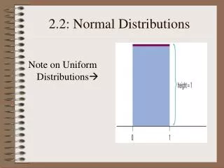
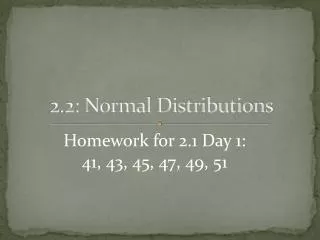
Section 2.2 Normal Distributions. Mrs. Daniel AP Statistics. Section 2.2 Normal Distributions. After this section, you should be able to… DESCRIBE and APPLY the 68-95-99.7 Rule DESCRIBE the standard Normal Distribution PERFORM Normal distribution calculations ASSESS Normality.

E N D
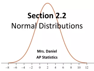
Section 2.2 Normal Distributions Mrs. Daniel AP Statistics
Section 2.2Normal Distributions After this section, you should be able to… • DESCRIBE and APPLY the 68-95-99.7 Rule • DESCRIBE the standard Normal Distribution • PERFORM Normal distribution calculations • ASSESS Normality
Normal Distributions • All Normal curves are symmetric, single-peaked, and bell-shaped • A Specific Normal curve is described by giving its mean µ and standard deviation σ. Two Normal curves, showing the mean µ and standard deviation σ.
Normal Distributions • We abbreviate the Normal distribution with mean µ and standard deviation σ as N(µ,σ). • Any particular Normal distribution is completely specified by two numbers: its mean µ and standard deviation σ. • The mean of a Normal distribution is the center of the symmetric Normal curve. • The standard deviation is the distance from the center to the change-of-curvature points on either side.
Normal Distributions are Useful… • Normal distributions are good descriptions for some distributions of real data. • Normal distributions are good approximations of the results of many kinds of chance outcomes. • Many statistical inference procedures are based on Normal distributions. Normal Distributions will appear AGAIN and AGAIN. Chapter 6, Chapter 8, Chapter 9 and Chapter 10!
The 68-95-99.7 Rule Although there are many different sizes and shapes of Normal curves, they all have properties in common. • The 68-95-99.7 Rule (“The Empirical Rule”) • In the Normal distribution with mean µ and standard deviation σ: • Approximately 68% of the observations fall within σ of µ. • Approximately 95% of the observations fall within 2σ of µ. • Approximately 99.7% of the observations fall within 3σ of µ.
The distribution of Iowa Test of Basic Skills (ITBS) vocabulary scores for 7th grade students in Gary, Indiana, is close to Normal. Suppose the distribution is N(6.84, 1.55) and the range is between 0 and 12. • Sketch the Normal density curve for this distribution.
The distribution of Iowa Test of Basic Skills (ITBS) vocabulary scores for 7th grade students in Gary, Indiana, is close to Normal. Suppose the distribution is N(6.84, 1.55) and the range is between 0 and 12. • Sketch the Normal density curve for this distribution.
The distribution of Iowa Test of Basic Skills (ITBS) vocabulary scores for 7th grade students in Gary, Indiana, is close to Normal. Suppose the distribution is N(6.84, 1.55). b) Using the Empirical Rule, what percent of ITBS vocabulary scores are less than 3.74?
The distribution of Iowa Test of Basic Skills (ITBS) vocabulary scores for 7th grade students in Gary, Indiana, is close to Normal. Suppose the distribution is N(6.84, 1.55). b) Using the Empirical Rule, what percent of ITBS vocabulary scores are less than 3.74?
The distribution of Iowa Test of Basic Skills (ITBS) vocabulary scores for 7th grade students in Gary, Indiana, is close to Normal. Suppose the distribution is N(6.84, 1.55).? c) Using the Empirical Rule, what percent of the scores are between 5.29 and 9.94?
The distribution of Iowa Test of Basic Skills (ITBS) vocabulary scores for 7th grade students in Gary, Indiana, is close to Normal. Suppose the distribution is N(6.84, 1.55).? c) Using the Empirical Rule, What percent of the scores are between 5.29 and 9.94?
Importance of Standardizing • There are infinitely many different Normal distributions; all with unique standard deviations and means. • In order to more effectively compare different Normal distributions we “standardize”. • Standardizing allows us to compare apples to apples. • We can compare SAT and ACT scores by standardizing.
The Standardized Normal Distribution All Normal distributions are the same if we measure in units of size σ from the mean µ as center. The standardized Normal distribution is the Normal distribution with mean 0 and standard deviation 1.
1. Draw and label an Normal curve with the mean and standard deviation. 2. Calculate the z- score x= variable µ= mean σ= standard deviation 3. Determine the p-value by looking up the z-score in the Standard Normal table. 4. Conclude in context. How to Standardize a Variable:
The Standard Normal Table Because all Normal distributions are the same when we standardize, we can find areas under any Normal curve from a single table. The Standard Normal table is a table of the areas under the standard normal curve. The table entry for each value “z” is area under the curve to the LEFT of z. The area to left is called the “p-value” • Probability • Percent
Using the Standard Normal Table Row: Ones and tenths digits Column: Hundredths digit Practice: What is the p-value for a z-score of -2.33?
Using the Standard Normal Table Using the Standard Normal Table, find the following:
Using the Standard Normal Table Using the Standard Normal Table, find the following:
Let’s Practice In the 2008 Wimbledon tennis tournament, Rafael Nadal averaged 115 miles per hour (mph) on his first serves. Assume that the distribution of his first serve speeds is Normal with a mean of 115 mph and a standard deviation of 6.2 mph. About what proportion of his first serves would you expect to be less than 120 mph? Greater than?
1. Draw and label an Normal curve with the mean and standard deviation. 2. Calculate the z- score x= variable µ= mean σ= standard deviation
3. Determine the p-value by looking up the z-score in the Standard Normal table. P(z < 0.81) = .7910
4. Conclude in context. We expect that 79.1% of Nadal’s first serves will be less than 120 mph. We expect that 20.9% of Nadal’s first serves will be greater than 120 mph.
Let’s Practice When Tiger Woods hits his driver, the distance the ball travels can be described by N(304, 8). What percent of Tiger’s drives travel between 305 and 325 yards?
When Tiger Woods hits his driver, the distance the ball travels can be described by N(304, 8). What percent of Tiger’s drives travel between 305 and 325 yards? Step 1: Draw Distribution Step 2: Z- Scores
Step 3: P-values Using Table A, we can find the area to the left of z=2.63 and the area to the left of z=0.13. 0.9957 – 0.5517 = 0.4440. Step 4: Conclude In Context About 44% of Tiger’s drives travel between 305 and 325 yards.
TI-Nspire: NormalCDF Normalcdf- “Area under the curve between two points” • Select Calculator (on home screen), press center button. • Press menu, press enter. • Select 6: Statistics, press enter. • Select 5: Distributions, press enter. • Select 2: Normal Cdf, press enter. • Enter the following information: • Lower: (the lower bound of the region OR 1^-99) • Upper: (the upper band of the region OR 1,000,000) • µ: (mean) • Ơ: (standard deviation) • Press enter, number that appears is the p-value
TI-Nspire: NormalPDF Normalpdf- “Exact percentile/probability of a specific event occurring” • Select Calculator (on home screen), press center button. • Press menu, press enter. • Select 6: Statistics, press enter. • Select 5: Distributions, press enter. • Select 1: Normal Pdf press enter. • Enter the following information: • Xvalue (not a percent) • µ: (mean) • Ơ: (standard deviation) • Press enter, number that appears is the p-value
TI-Nspire: InvNorm invNorm- “Exact x-value at which something occurred” • Select Calculator (on home screen), press center button. • Press menu, press enter. • Select 6: Statistics, press enter. • Select 5: Distributions, press enter. • Select 3: Inverse Norm press enter. • Enter the following information: • Area (enter as a decimal) • µ: (mean) • Ơ: (standard deviation) • Press enter, number that appears is the p-value
When Tiger Woods hits his driver, the distance the ball travels can be described by N(304, 8). What percent of Tiger’s drives travel between 305 and 325 yards?
When Tiger Woods hits his driver, the distance the ball travels can be described by N(304, 8). What percent of Tiger’s drives travel between 305 and 325 yards?
Suzy bombed her recent AP Stats exam; she scored at the 25th percentile. The class average was a 170 with a standard deviation of 30. Assuming the scores are normally distributed, what score did Suzy earn on the exam?
Suzy bombed her recent AP Stats exam; she scored at the 25th percentile. The class average was a 170 with a standard deviation of 30. Assuming the scores are normally distributed, what score did Suzy earn of the exam?
Whenever the distribution is Normal. • Ways to Assess Normality: • Plot the data. • Make a dotplot, stemplot, or histogram and see if the graph is approximately symmetric and bell-shaped. • Check whether the data follow the 68-95-99.7 rule. • Construct a Normal probability plot. When Can I Use Normal Calculations?!
Normal Probability Plot • These plots are constructed by plotting each observation in a data set against its corresponding percentile’s z-score.
Interpreting Normal Probability Plot • If the points on a Normal probability plot lie close to a straight line, the plot indicates that the data are Normal. • Systematic deviations from a straight line indicate a non-Normal distribution. • Outliers appear as points that are far away from the overall pattern of the plot.
MC #1 Scores on the ACT college entrance exam follow a bell-shaped distribution with mean 18 and standard deviation 6. Wayne’s standardized score on the ACT was −0.7. What was Wayne’s actual ACT score? (a) 4.2 (b) −4.2 (c) 13.8 (d) 17.3 (e) 22.2
MC #2 Which of the following is least likely to have a nearly Normal distribution? (a) Heights of all female students taking STAT 001 at State Tech. (b) IQ scores of all students taking STAT 001 at State Tech. (c) SAT Math scores of all students taking STAT 001 at State Tech. (d) Family incomes of all students taking STAT 001 at State Tech. (e) All of (a)–(d) will be approximately Normal.
MC #3 The scores on the real estate licensing exam given in Florida are Normally distribution with a standard deviation of 70. What is the mean test score if 25% of the applicants score above 475? • 416 b. 428 c. 468 d. 522 e. Not enough information to answer question.
MC #4 Polly takes three standardized tests. She scores 600 on all three tests. The scores are Normal distributed. Rank her performance on the three tests. • I, II and III b. III, II, and I c. I, III and II d. III, I, and II e. II, I and III
MC #5 The heights of American men aged 15 to 24 are approximately normally distributed with a mean of 68 inches and a standard deviation of 2.5 inches. About 20% of these men are taller than… a. 66 inches b. 68 inches c. 70 inches d. 72 inches e. 74 inches
MC #6 Which of the following variables would most likely follow a Normal model? • Family income • Heights of singers in a co-ed choir • Weight of adult male elephants • Scores on an easy test • All of these
MC #7 Suppose that a Normal model described student scores in a history class. Parker has a standardized score (z-score) of +2.5. This means that Parker • Is 2.5 points above average for the class. • Is 2.5 standard deviations above average for the class. • Has a standard deviation of 2.5. • Has a score that is 2.5 times the average for the class. • None of the above.
MC #8 Suppose a Normal model describes the number of pages printer ink cartridges last. If we keep track of printed pages for the 47 printers at a company’s office, which must be true? • The page counts for those ink cartridges will be normally distributed. • The histogram for those page counts will be symmetric. • 95% of those page counts will be within 2 standard deviation of the mean. • None B. I only C. II only D. II and III E. I, II and III
Summary: Normal Distributions • The Normal Distributions are described by a special family of bell-shaped, symmetric density curves called Normal curves. The mean µ and standard deviation σ completely specify a Normal distribution N(µ,σ). The mean is the center of the curve, and σ is the distance from µ to the change-of-curvature points on either side. • All Normal distributions obey the 68-95-99.7 Rule, which describes what percent of observations lie within one, two, and three standard deviations of the mean. • All Normal distributions are the same when measurements are standardized. The standard Normal distribution has mean µ=0 and standard deviation σ=1. • Table A gives percentiles for the standard Normal curve. By standardizing, we can use Table A to determine the percentile for a given z-score or the z-score corresponding to a given percentile in any Normal distribution. • To assess Normality for a given set of data, we first observe its shape. We then check how well the data fits the 68-95-99.7 rule.
Finding Areas Under the Standard Normal Curve Find the proportion of observations from the standard Normal distribution that are between -1.25 and 0.81. Step 1: Look up area to the left of 0.81 using table A. Step 2: Find the area to the left of -1.25