Download
1 / 8
80 likes | 151 Views
Explore various programs aiding accelerator physicists in designing and building accelerators. Examples range from electromagnetics to particle tracking. Discover how models are utilized in practical accelerator simulations and analyses.

E N D
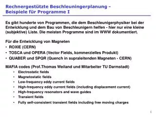
Rechnergestützte Beschleuningerplanung -Beispiele für Programme I • Es gibt hunderte von Programmen, die dem Beschleunigerphysiker bei der Entwicklung und dem Bau von Beschleunigern helfen - hier nur eine kleine (subjektive) Liste. Die meisten Programme sind im WWW dokumentiert. • Für die Entwicklung von Magneten • ROXIE (CERN) • TOSCA und OPERA (Vector Fields, kommerzielles Produkt) • QUABER und SPQR (Quench in supraleitenden Magneten - CERN) • MAFIA codes (Prof.Thomas Weiland und Mitarbeiter TU Darmstadt) • Electrostatic fields • Magnetostatic fields • Low-frequency eddy current fields • High-frequency eddy current fields (including displacement current) • High-frequency resonators and wave guides • Transient fields • Fully self-consistent transient fields including free moving charges
Beispiele für Programme II • Mechanik + Dynamische Systeme • ANSYS (Finite Elemente) • Simulation needs encompass structural, contact, thermal, computational fluid dynamics (CFD), acoustics, electrostatics, magnetostatics, and low- or high-frequency electromagnetics capabilities • Beschleunigeroptik • MAD (CERN) • Trackingprogramme in diversen Labors, z.B. Sixtrack (CERN) • Korrektur des Teilchenbahn (COCU - CERN) • Wechselwirkung von Teilchen mit Materie • GEANT (CERN + outside) • EGS • FLUKA (CERN)
Beispiele für Programme III • Viele Programme, die für andere Anwendungen entwickelt worden, kommen in der Beschleunigerphysik und Technik zu Anwendung. Beispiele sind: • Mathematik • Mathematica • MathCad • Elektronik • PSPICE • PCAD • Messtechnik • LABVIEW • Zeichnungen und virtuelle Realität • AUTOCAD • EUCLID • Ausserdem gibt es noch unzählige Programme an den verschiedenen Beschleunigerinstituten, die für spezielle Anwendungen geschrieben wurden.
Modellbeschleuniger • Anstatt Details über die verschiedenen Programme zu diskutieren: • Praktisches Beispiel für den Modellbeschleuniger in MATHCAD • Lineare Optik • Betatronschwingungen • Emittanz • Nichtlinearität • Tracking • Synchrotronschwingungen • Spektrum des Strahls
Modellbeschleuniger: transversaler Phasenraum • Lineare Optik: • k=1.4195 qx=ganzzahlig tune = 1 • (wenn man 4 Zellen hat, wird der tune halbzahlig) • k=1.43 qx=1.022 • k=1.44 qx=1.044 • k=1.48 qx=1.137 • k=1.50 qx=1.188 • k=1.51 qx=1.228 • k=1.52 qx=1.242 • k=1.55104 qx=1.333 • sextupole 0.001 = starts to be instable, instable at 512 turns • k=1.50 qx=1.188 stable again • k=1.50 qx=1.188 sextupole 0.050 stable but distorted phase space
Modellbeschleuniger: longitudinaler Phasenraum • Beispiel 1: fs = 0.125 und As=1, eine Periode in 4 Umläufen, und in der Frequenz sieht man einen peak bei 512 • Beispiel 2: wie 1, mit As=10, man nur bei einigen Umläufen ein Signal, immer dann, wenn der Bunch im Zentrum ist (alle 4 Umläufe, fuer 180 und 360 Grad) • Beispiel 3: f2=0.120 und As=0.2 - nur ein Peak • Bespiel 4: wie 3, und As=1 - 2ter Peak sehr klein • Beispiel 5: wie 3 und As=2, 2ter Peak, und 3ter Peak • Beispiel 6: fs=0.0125 und As=2
Modellbeschleuniger: Bunchspektrum • 1 Bunche, 0.5 ns, bis 200 • 1 Bunche, 0.1 ns, bis 200 • 10 Bunche, 0.1 ns, bis 200
F0D0 Zelle des Modelspeicherrings QF Dipol QD Dipol QF lB=1.50 m lq=0.40 m lB=1.50 m ld=0.55 m F0D0 Zelle MQF MB MQD MQD MB MQF MD1 MD1 MD1 MD1 MEB MEB MEB MEB