Download
1 / 42
420 likes | 653 Views
Evaluating Mass Flux Closures Using Cloud Resolving Model Simulations of Deep Convection. Evaluating mass flux closures using cloud resolving model simulations of deep convection. Jennifer Fletcher and Chris Bretherton COGS talk May 7, 2009.

E N D
Evaluating Mass Flux Closures Using Cloud Resolving Model Simulations of Deep Convection Evaluating mass flux closures using cloud resolving model simulations of deep convection Jennifer Fletcher and Chris Bretherton COGS talk May 7, 2009 Jennifer Fletcher and Chris Bretherton COGS presentation May 7, 2009
What does cumulus convection do? • Makes precipitation and severe weather • Changes stability • Generates and redistributes heat and moisture • Transports tracers • Makes clouds that affect radiation Cumulus parameterizations must represent some or all of these effects
Two basic types of cumulus parameterization: adjustment and mass flux • Adjustment: temperature and moisture adjust to pre-specified profiles over a finite timescale. • Mass flux: a cloud model explicitly calculates profiles of cumulus mass flux and thermodynamic variables. • Mass flux more widely used because it can provide an internally consistent representation of turbulent mixing, updraft dynamics, microphysics, and tracer transport
Three components to a mass flux parameterization • Trigger: will convection occur? • Closure: how much convection? • Model: how will convection distribute heat, moisture, etc? The trigger and the closure may be considered two parts of the same thing
Mass flux parameterization • The closure relates the cloud base mass flux to resolved-scale variables • A cloud model predicts the vertical structure of mass flux and thermodynamic quantities above cloud base • My research focuses on a type of mass flux closure Cloud model predicts cumulus properties per cloud base mass flux mcb = f(large scale)
What I am going to show you • Mass flux closure based on convective inhibition (CIN) is well suited for both shallow and deep convection. • This closure takes the form mcb=c1Wexp(-c2CIN/TKE) • W is a vertical velocity scale • TKE = mean turbulent kinetic energy in the boundary layer
Mass flux closure: fundamental assumptions • Cumulus cloud base mass flux is a function of large scale variables • Cloud base mass flux has no memory, i.e., it is determined by instantaneous forcings.
Mass flux closure types • Moisture convergence • CAPE • Boundary layer based
Mass flux closure type 1: moisture convergence • Mass flux determined so that precipitation balances moisture convergence, as observed over the tropical oceans. • Lacking in causality: convection can’t see moisture convergence & must ultimately respond to local thermodynamic profile • Performs poorly if the storage term in the moisture budget is significant on convective time scales (e.g., continental convection). • Examples: Kuo, Anthes • Popular in the 80’s but has largely fallen out of favor.
Mass flux closure type 2: CAPE • Cumulus base mass flux depends on the vertically-integrated parcel buoyancy (adiabatic or entraining) • Causality issue: how can cloud base mass flux feel the deep updraft buoyancy profile? • CAPE and cloud base mass flux are inconsistently correlated in tropical oceanic convection. • Widely used, e.g.,Arakawa-Schubert (GFS, GFDL), Zhang-McFarlane (CAM), Kain-Fritsch (WRF) From Kuang and Bretherton (2006)
Mass flux closure type 3: boundary layer (BL)-based • Defining characteristic: PBL quantities (e.g., surface fluxes, CIN, TKE) determine cloud base mass flux. • Motivation: the roots of cumulus updrafts are in the boundary layer. • Applicable to shallow as well as deep convection • Example: UW shallow cumulus scheme (CAM)
BL closure I: CIN closure Concept: mcb controlled by KE of PBL updrafts and their potential energy barrier (CIN). Introduced by Mapes (2000) • mcb= c1Wexp(-c2CIN/W2) • Distribution of CIN & W • Acts as a trigger as well Plan view of PBL vertical velocity (gray positive) in LES. From Moeng and Rotunno (1990)
mcb = c1Wexp(-c2CIN/W2) CIN closure maintains an important feedback • Keeps PBL top near cloud base • If PBL top above LCL, CIN small, lots of convection, lowers PBL height • If PBL top far below, lots of CIN, no convection, PBL ht increases due to sfc fluxes & entrainment p LCL PBL top ave z ~1K =(1 + 0.61qv-qc)
BL closure II: Grant closure • Grant and Brown (1999) found in an LES that mcb ~ 0.03w* • w* = (B0zPBL)1/3 - the PBL convective velocity scale. • Attractively simple but still requires a trigger. • This diagnostic relationship is used as a closure in the UW shallow convection scheme as implemented in the GFDL model.
Testing BL-based closure • Strategy: use a cloud resolving model to test • CIN [mcb=c1Wexp(-c2CIN/W2) ] and • Grant (mcb=0.03w*) closures, which were developed for shallow convection. • Test these closures for deep convection. • Methods: • Use several different CRM simulations • Calculate the cloud base cumulus mass flux mcb. • Test relationships between mcb and PBL variables predicted by closure
Issues with this approach • 1. Analyzing instantaneous 3-D volumes gives sampling uncertainty • 2. Use of large-scale forcings constrains convection. • But this constraint is identical to that under which a cumulus parameterization operates. -500 200 Julian Day 260
System for Atmospheric Modeling (SAM) Solves the anelastic equations, 3D geometry, bulk microphysics, periodic lateral BC’s Simulated satellite image during KWAJEX Source: http://rossby.msrc.sunysb.edu/%7Emarat/SAM.html See Khairoutdiov and Randall (2003)
SAM simulations • Use well-verified simulations of three intensive observing periods • ARM (Atmospheric Radiation Measurement) Oklahoma site, summer 1997 • KWAJEX (Kwajalein Experiment) in West Pacific ITCZ, summer 1999 • BOMEX (Barbados Oceanography and Meteorology Experiment) in trade Cu environment, June 1969
SAM simulations: ARM (Oklahoma, late June 1997) • SAM version 6.7 • 192x192 km2 domain, x = 1 km • 96 vertical grid levels, z ranges from ~50-100 m in PBL to 250 m in free troposphere, larger above tropopause. • 15 days long • Features a range of conditions including clear sky, shallow convection, and episodic deep convection See Khairoutdiov and Randall (2003)
SAM simulations: KWAJEX (West Pacific ITCZ) • SAM version 6.3 • 50 days • 256x256 km2 domain, x = 1 km • 64 vertical grid levels, z ranges from 100 m in PBL to 400 m in free troposphere, larger above tropopause. • Continuously-forced tropical marine deep convection. See Blossey et al (2007)
SAM simulations: BOMEX (trade cumulus regime) • SAM version 6.7 • 6 hours • 192x192x96 grid points • x = z = 40 m everywhere. • Steadily-forced subtropical shallow cumulus convection. • Non-interactive radiative cooling profile. See Siebesma et al (2003)
SAM simulations: Cloud Fraction Note different color & vertical scales!
mcb = c1Wexp(-c2CIN/W2) What I need to test CIN closure • A definition of cumulus (Cu) updraft: saturated pixel with w > 0.5 m/s • An estimate of Cu updraft base • Cu- base updraft mass flux • Average CIN that Cu-base updrafts have overcome • A vertical velocity scale for Cu updrafts (call this W)
Methods: finding cloud base • Define one representative Cu base height. • Use a profile-based approach that is consistent with what a GCM can do. • Approach:Find lifting condensation level (LCL) of a test parcel with similar thermodynamic properties to Cu updrafts. • Parcel originating at 300 m ‘spiked’ with 1 horizontal std (q) of qv works well. • Cloud reference level: 1st grid level above this LCL.
Cloud reference level & Cu updraft fraction Cloud reference level captures Cu base very well
Analyzing Cu-base mass flux • Use cloud reference level as proxy for cloud base. • Mass flux Mcb = cbwcb • cb = cloud ref level Cu updraft fractional area. • wcb = Cu updraft vertical velocity • We often use mcb=Mcb/ ([mcb] = m/s) • We’ll analyze the vertical velocity and cloud fraction contributions to mass flux separately.
Cu base mass flux shows considerable variability & is somewhat correlated with precip • But times when no precip & plenty of Cu base mass flux • 600 hPa mass flux much better correlated with precip Cu updraft mass flux 600 hPa mass flux hello Cld ref level mass flux
mcb = c1Wexp(-c2CIN/W2) Calculating cloud ref level CIN Example KWAJEX day, rain rate = 5mm/hr 900 • At cloud ref level, calculate mean T and qT of Cu updrafts. • Adiabatically displace to ~300m • b(z) = gT’/Tave Sounding T cloud ref level Ave Cu updraft T Wowwowsa wowsa Actual cloud base 200
mcb = c1Wexp(-c2CIN/W2) Calculating Cu-updraft vertical velocity scale W • Two possibilities I considered: TKE1/2 and w* • TKE = 1/2(u’2 + v’2+w’2), PBL large eddies + cold pool dynamics • w* (implicated by Grant) depends on surface fluxes and BL depth. • In a dry convective BL, the two are linearly related. • Compare these to wcb,, the actual vertical velocity of Cu updrafts at cloud ref level.
CIN, TKE, w* TKE1/2 CIN1/2 • TKE correlated w/ precip. • CIN & TKE covary • Cu-base velocity wcb looks like TKE1/2 for KWAJEX, w* for ARM w* wcb wcb
mcb = c1Wexp(-c2CIN/W2) Cu-base vertical velocity scale W • Try W = aw* + bTKE1/2 • Choose a & b to minimize sum of (W-wcb)2 over all times for ARM, KWAJEX, and BOMEX wcb [m/s]
mcb = c1Wexp(-c2CIN/W2) Cu-updraft fractional area • General form: • cb=c1exp(-c2CIN/W2) • But CIN/W2 is often much too large • CIN/TKE is a much better predictor • Reflects role of cold pools? Implied by Grant closure
mcb = c1Wexp(-c2CIN/TKE) W = aw* + bTKE1/2 Combined results: mass flux closure Closure skillfully predicts Cu-base mass flux, subject to substantial sampling uncertainty actual closure
Can a GCM implement this closure? • We used CIN of conditionally sampled cu-updrafts and the actual BL-mean TKE in these calculations. • How can this be implemented in a GCM? 1: TKE can be calculated from a combination of w* and precipitation. 2: CIN can be calculated from the sounding…
Estimating Cu-updraft CIN from the sounding • As before, start a parcel at ~300m with domain mean and qv=qvmean+qv. • Lift parcel adiabatically to cloud reference level. • The CIN of this parcel is well-correlated with the CIN of cloud reference level Cu-updrafts.
CIN closure using sounding CIN • Calculating CIN from the sounding still produces a skillful estimate of Cu-base mass flux. • How to represent TKE and qv std are left as open questions. actual closure CIN estimated from sounding
Conclusion CIN closure mcb=0.03Wexp(-CIN/TKE) with Cu-base updraft velocity W = 0.57w*+0.24TKE1/2 skillfully predicts cloud base mass flux for a range of realistic CRM simulations of shallow and deep convection.
Future work • To complete the closure, determine how to parameterize q and TKE (Cathy Hohenegger). • These can be specified in terms of surface fluxes, precipitation, mean RH, and vertical gradient in MSE.
Thank you Thanks also to Peter Blossey!
Boundary Layer closure I: BLQ • Boundary Layer quasi-equilibrium: proposed by Raymond (1995) for tropical oceanic deep convection • Closure assumption: convection keeps PBL e near a “convective threshold” • Surface fluxes increase PBL e while convective downdrafts decrease it • Not applicable to shallow or continental deep convection Low e downdraft ePBL~ ethresh flux of high esurf