Simple Group Comparisons
Simple Group Comparisons. Limits you to simple explanatory variables simple potential relationships. Complex Group Difference Designs. Types Multilevel Designs – single IV, 3 or more levels Single source of possible systematic variability, but more than a simple difference possible

Simple Group Comparisons
E N D
Presentation Transcript
Simple Group Comparisons Limits you to simple explanatory variables simple potential relationships
Complex Group Difference Designs Types Multilevel Designs – single IV, 3 or more levels Single source of possible systematic variability, but more than a simple difference possible Multifactor Designs (Factorial) – multiple IVs Multiple possible sources of systematic variability Not all effects have single variable causes
Multilevel Designs Situations requiring a multilevel approach Characteristics of the IV appropriate representation of IV variability Level of Sense of Humor and Perceived Personality No two levels of SoH are likely to represent important differences Characteristics of the IV DV relationship a nonlinear relationship anticipated Level of Test Anxiety and Test Performance Would not expect a linear relationship
Multilevel Designs Evaluating the Results – searching for the systematic variability in the DV no single place (difference) to assess, variability could appear in multiple places - examples or in multiple forms - examples
Multilevel Designs Two common approaches Overall test for ‘systematic variability’ - with follow-up (post hoc) tests to see where differences ‘might’ exist (Means vary systematically, as opposed to no more than unsystematically) Test for ‘fit’ with predicted pattern across groups Using planned comparisons or ‘contrasts’ to specify pattern (Means vary systematically in a predicted form or pattern)
Multilevel Designs Overall test for ‘systematic variability’ Ho: M1 = M2 = M3………… variability among sample means will be no greater than variability expected due to unsystematic variability Possibly two steps in the analysis 1. Test to see if Ho can be rejected If yes, there is evidence of systematic variability 2. Examine differences between means to see where systematic variability occurs
Multilevel Designs Test for ‘fit’ to predicted pattern across groups Ho: M1 = M2 = M3………… Specify pattern expected (contrast) and test to see if systematic variability does ‘fit’ that pattern - allowed as many ‘orthogonal’ contrasts as there are df overall - if doing nonorthogonal contrasts, may need to adjust Type 1 L = S cM, where c is the ‘weight’ assigned to each mean to represent the pattern predicted (and add up to 0)
Multilevel Designs Test for ‘fit’ to predicted pattern across groups Ho: M1 = M2 = M3………… Specify pattern expected (contrast) and test to see if systematic variability does ‘fit’ that pattern Contrast to test linear relationship between Sense of humor and Liking as SOH goes up, Liking goes up Contrast to test curvilinear relationship between Test Anxiety and outcome low and high anxiety lower the outcome, relative to moderate
Multifactor Designs Situations requiring a Multifactor approach multiple possible Causes (each sufficient, not necessary) more efficient to assess in a single design laugh at your joke (or not) similar attitudes (or not) interactions among Causes needed to produce effect (necessary, not sufficient causal influence) high choice in behaving counter to one’s attitude (vs low choice) high consequences for behavior (vs low consequences) need both to be High to get effect assess possible role of an EV in affecting DV psychological vs physical disorder (IV) gender or worker with disorder (EV)
Multifactor Designs Main Effects vs. Interaction Effects Main effects – relationship of each IV with the DV -one possible main effect for each IV in the design Interaction effects – combinations of levels of different IVs -effect of changes in one IV (on DV) depends upon level of another IV present
Multifactor Designs Understanding Multifactor Design notation How many main effects and interactions? 2 x 2 design - Chant (2) x Program (2) Kumbaya vs Chant 2 x 4 design – Program (2) x Chant (4) None, Kumbaya, Stats 1, Stats 2 2 x 2 x 3 design – Program (2) x Gender (2) x Chant (3) Kumbaya, Stats 1, Stats 2
Multifactor Designs What if the groups have unequal n’s? What is being compared? Numbers that represent main effects and interactions main effects in ‘margins” interactions ‘inside’ look at some examples with Means 2 x 2 design 2 x 4 design 2 x 2 x 3 design
Multifactor Designs Following up on significant main effects and interactions Multilevel main effects Simple main effects in interactions
Multifactor Designs Interpreting results when there are significant main effects and interaction effects Interactions take precedence in interpretations
Complex Group Difference Designs Independent Levels vs.Related Levels Independent Variables in Complex Group Designs Independent Levels Multilevel Related Levels Multilevel Independent Levels Multifactor Related Levels Multifactor Mixed Multifactor
Now – for the analyses Recall Variance = S(x-M)2 df Allows you to combine all the different deviations from the Mean to get a Sum (of squares), and then to find the ‘typical’ deviation (squared) by dividing by df
Evaluating Results in Complex Group Difference Designs – Interval/Ratio Data Need to be able to assess multiple possible differences that might reflect “systematic” variability along a single dimension - Multilevel Variables/Designs and/or could be the result of multiple independent sources of ‘systematic’ variability – Multifactor Designs
t = Building from the t-test single deviation (M – M) typical deviation (se) Numerator could be treated as two deviations Group 1 mean – Population mean (estimated) Group 2 mean – Population mean (estimated) Sum the deviations (after squaring), and find the ‘average’ (what do you have?)
Building from the t-test single deviation (treat as 2 deviations from Mean) typical deviation (square to convert to variance) Now you could compare that ‘variance’ (numerator) (may be due to a situation where Ho is not true) to the typical variance (when Ho true) by squaring the denominator
t = Building from the t-test (based on deviations) single deviation (systematic and unsystematic) typical deviation unsystematic F statistic – from Analysis of Variance Variance (systematic and unsystematic) Variance unsystematic F =
F = When you have only two groups, F = t2, but now, with F, you can include any number of means in the numerator of the F-ratio. What you have is: estimate of population variance estimate of population variance One estimate is sensitive to systematic variability One estimate is unaffected by systematic variability
population Sample 1 IV level 1 Sample 2 IV level 2 Sample 3 IV level 3 Want to ‘estimate’ variance in the population Sample variance 3 Sample variance 1 Sample variance 2 Most logical strategy is to use the variances from your samples to estimate the variance in the population.
population Sample 2 IV level 2 Sample 3 IV level 3 Sample 1 IV level 1 Want to ‘estimate’ variance in the population Sample mean 3 Sample mean 1 Sample mean 2 Can also estimate the population variance by using means from samples, but this estimate will only be accurate when the Ho is true
F = estimate of population variance using means estimate of population variance using variances Means are sensitive to systematic variability Variances are unaffected by systematic variability systematic + unsystematic variability unsystematic variability F =
Variance = Analysis of Variance involves ‘partitioning’ the variability of the DV into the variability relevant to the parts of the F ratio. Recall that: Sum of Squares df So the ‘sum of squares’ reflects the variability of DV (before it is ‘averaged’) Some of the variability (sum of squares) reflects only unsystematic variability Some of the variability (sum of squares) reflects systematic + unsystematic variability
Partitioning the Sum of Squares (in a balanced design) Two groups (for simplicity) Non chanters (25) Chanters (25)
x All 50 students as a sample SSTotal – sum of the squared deviations of individual scores from the mean of the entire sample – ignoring group membership ‘Sample Mean’ SSWithin – sum of the squared deviations of individual scores from the mean of the individual’s group, based on variability within each group Students divided by Level of IV ‘Group Mean’ ‘Group Mean’ SSBetween – sum of the squared deviations of typical score from group from the mean of the entire sample – treats individuals as if they are ‘typical’ for their group Students as ‘typical’ members of their group When equal n, SST = SSW + SSB ‘Group Mean’ ‘Group Mean’ ‘Sample Mean’
Evaluating Results in Complex Group Difference Designs – Interval/Ratio Data SST = S(x – MG)2 as if one group of participants SSW = S(xg1 – Mg1)2 variability within each + S(xg2 – Mg2)2 group – relative to + S(xg3 – Mg3)2 each group’s mean SSB = n(Mg1 – MG)2 variability among group + n(Mg2 – MG)2 means, relative to the + n(Mg3 – MG)2 mean of the entire sample
Evaluating Results in Complex Group Difference Designs – Interval/Ratio Data Analysis of Variance Assumptions 1. Interval/ratio data 2. Independent observations 3. Normal sampling distribution of the means (seldom a problem) 4. Homogeneity of variances (same guidelines as for t-test)
Example – multilevel design IV is Sense of Humor of Target Person (3 levels: Below Ave - Average - Above Ave) DV is rated liking, from low (1) to (7) high 4 participants per group (power = .09) Levels of Sense of Humor of Target Below Ave Average Above Ave Means 2 4 6 Variances .67 .67 .67
Deviations of Group Means from Sample Mean Deviations within each group from group mean Deviations from Overall Sample Mean
Rating 7 Group mean 6 5 Overall sample mean 4 3 2 1 1 2 3 4 5 6 7 8 9 10 11 12 Below Average Average Above Average Subjects
Mean Square Between = Sum of Squares Between/dfbetween (estimate of population variance based upon Means) Mean Square Within = Sum of Squares Within/dfwithin (estimate of population variance based upon group Variances) MSB -- biased estimate MSW -- unbiased estimate ?? Does the variability among the means (relative to the estimated population mean) appear to be greater than the variability expected when the Null Hypothesis is true (error variability only)? F (dfb, dfw) = F (dfb, dfw) =
The variance in each group is .81652 or .667 – the same as the MSW in the Table below Since this is the best estimate of the population variance If we assume each person’s rating in a group was equal to the mean (typical) rating for that group, the estimated population variance is the MSB (ivsoh) Power to detect a moderate effect (eta2 of 6%) = .09 NOT Partial SSB SSW SST eta2 = SSB/SST Why are these the df’s
Go through the steps in SPSS Analyze General Linear Model Univariate Choose DV Choose IV (Fixed Factor) Options Estimated Marginal Means only needed in Multifactor Designs Must use for Main Effects if unequal n in cells Can use Pairwise Comparisons to get CI’s for Main Effects Descriptive Statistics Estimates of Effect Size Homogeneity Tests Post hoc Choose as desired Can reset the alpha level in Options
Examples in Handouts Multilevel ANOVA “Multilevel” Chi square
Multilevel Designs Situations requiring a Multilevel approach - single IV in the design – 3 or more levels SST = SSW + SSBiv MSB MSW F (dfb, dfw) =
Multifactor Designs Situations requiring a Multifactor approach - including multiple IVs in the design so for the 2 x 2 multifactor design SST = SSW + SSBiv becomes SST = SSW + SSBiv1 + SSBiv2 + SSBinteraction To answer 3 questions
Independent Variable 1 – Music Level 1 = Rock Level 2 = ClassicalIndependent Variable 2 = Volume Level 1 = Low Level 2 = HighDependent Variable = Number of words recalled from a list of 20. Power = .18 For eta2 = .06 (moderate effect) • Independent Variable 1 • MUSIC • Rock Classical_ _ _ • 13 8 • 10 5 sum = 90 • Level 1 9 M = 10 11 M = 8 • Low 7 8 M = 9 • 11 8 • Independent Variable 2 ___________________________ ____ • VOLUME 19 3 • 16 6 sum = 110 • Level 2 18 M = 16 9 M = 6 • High 13 6 M = 11 • 14 6 • _________________ _______ _______ • sum = 130 sum = 70 sum = 200 • M = 13 M = 7 Ms = 10 • Overall Sample Mean
(1) (2) SSW (4) SST (6) SSB || (1) (2) SSW (4) SST (6) SSB Xi (Xi-Mg) (Xi-Mg)2 (Xi-MS) (Xi-MS)2 (Mg-MS) (Mg-MS)2 Xi (Xi-Mg) (Xi-Mg)2 (Xi-MS) (Xi-MS)2 (Mg-MS) (Mg-MS)2 13 13-10 9 13-10 9 10-10 0 || 8 8-8 0 8-10 4 8-10 4 10 10-10 0 10-10 0 10-10 0 || 5 5-8 9 5-10 25 8-10 4 9 9-10 1 9-10 1 10-10 0 || 11 11-8 9 11-10 1 8-10 4 7 7-10 9 7-10 9 10-10 0 || 8 8-8 0 8-10 4 8-10 4 11 11-101 11-10 110-100 || 88-808-10 48-10 4 50 0 20 0 20 0 0 || 40 0 18 -10 38 -10 20 |G1 G2|__________________________________________________ ---------------------------------------------------|G3 G4|--------------------------------------------------- 19 19-16 9 19-10 81 16-10 36 || 3 3-6 9 3-10 49 6-10 16 16 16-16 0 16-10 36 16-10 36 || 6 6-6 0 6-10 16 6-10 16 18 18-16 4 18-10 64 16-10 36 || 9 9-6 9 9-10 1 6-10 16 13 13-16 9 13-10 9 16-10 36 || 6 6-6 0 6-10 16 6-10 16 1414-16414-101616-1036 || 66-606-10166-1016 80 0 26 30 206 30 180 || 30 0 18 -20 98 -20 80 SST = S(Xi – MS)2 SST = 20 + 38 + 206 + 98 = 362 SSW = S(Xig1 – Mg1)2 + S(Xig2 – Mg2)2+ S(Xig3 – Mg3)2 + S(Xig4 – Mg4)2 SSW = 20 + 18 + 26 + 18 = 82 SSBIV1 = n(Mgl+g3 – MS)2 + n(Mg2+g4- MS)2 SSBIV1 = 10(13-10)2 + 10(7-10)2 = 180 SSBIV2 = n(Mg1+g2 – MS)2 + n(Mg3+g4 – MS)2 SSBIV2 = 10(9-10)2 + 10(11-10)2 = 20 SSBX = SSB – SSBIV1 – SSBIV2 SSBX = 280 – 180 – 20 = 80
ANALYSIS OF VARIANCE TABLE • SourceSSdfMSF partial eta2 • Total 362 19 • Between • Music 180 1 180.00 35.12 .687 • Volume 20 1 20.00 3.90 .196 • Interaction 80 1 80.00 15.61 .494 • Within 82 16 5.125 • Critical F(1,16) = 4.49, p< .05, two-tailed test. • Partial eta2 SSB/(SSB+SSW)eta2 SSB/SST • Music 180/(180 + 82) = .687 180/362 = .497 • Volume 20/(20 + 82) = .196 20/362 = .055 • Interaction 80/(80+82) = .494 80/362 = .221 • Total 1.377 .773
Follow up analyses that might be needed with Multifactor Analyses If Multilevel IV main effect is significant need Multiple Comparison Tests Note – if unbalanced design, use tests available in Options to insure unweighted means are used If Interaction is significant need Simple Main effects tests which could include Multiple Comparisons Go to handouts for examples
Repeated Measures Multilevel Design Assumptions interval/ratio data independent observations (‘relatedness removed’) normality of sampling distribution homogeneity of variances of difference scores (sphericity) violations of homogeneity can be serious, and inflate the F values in post hoc tests, may want to use conservative test
Research – testing 3 separate recipes for Chocolate Chip Cookies IV Cookie Recipe – 3 levels DV Rated taste 1 2 3 4 5 6 7 8 9 Awful Delicious 5 participants, each tastes and rates each cookie (design issues?) cookie-a cookie-b cookie-c Means for Ps p1 5 7 9 7 p2 3 5 7 5 p3 1 3 8 3 p4 3 7 8 6 p5 5 7 9 7 Mcookie 3.4 5.8 8.2 5.8 Main effect for Participants – reflects differences across the participants Main effect for Cookie
Examples of SPSS in Handouts Show how to define RM variables in SPSS
Mixed Designs Combines aspects of both types (independent levels and related levels) but the error (MSW) used depends on whether the ‘effect’ is: truly independent levels, or related levels that have been ‘adjusted’ Assumptions interval ratio data normality of the sampling distribution independent observations for independent levels effects – homogeneity of variances for related levels effects – homogeneity of variances of difference scores (sphericity)
Mixed example Cookie Recipe (2) x Temperature (2) [ x Participants (n per group)] DV Rated taste Awful 1 2 3 4 5 6 7 8 9 Delicious Two cookies tasted by each person - within subjects effect some get warm cookies (n = 5), - between subjects effect some get room temperature (cold) cookies (n = 5), Warm Cold Cookie 1 Cookie 2 M Cookie 1 Cookie 2 M 1 5 7 6 3 5 4 2 6 8 7 4 7 5.5 3 8 7 7.5 3 5 4 4 6 8 7 3 5 4 5 6 8 7 4 6 5 6.2 7.6 6.9 3.4 5.6 4.5 2 x 2 Mixed Multifactor (treated as if 2 x 2 x 5) – but ignore Participants effects Partition SS into SSB – uncontaminated by relatedness SSB (Temperature – 2 levels) SSW (Participants within groups – variability among means of participants) SSW – systematic, but contaminated by relatedness SSB (cookies – 2 repeated measures levels) SSB interaction (2 x 2) SSW variability among participants