Download
1 / 31
310 likes | 461 Views
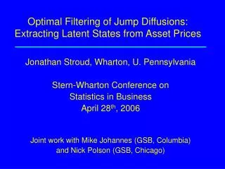
Optimal Filtering of Jump Diffusions: Extracting Latent States from Asset Prices. Jonathan Stroud, Wharton, U. Pennsylvania Stern-Wharton Conference on Statistics in Business April 28 th , 2006 Joint work with Mike Johannes (GSB, Columbia) and Nick Polson (GSB, Chicago). Overview.

E N D
Optimal Filtering of Jump Diffusions: Extracting Latent States from Asset Prices Jonathan Stroud, Wharton, U. Pennsylvania Stern-Wharton Conference on Statistics in Business April 28th, 2006 Joint work with Mike Johannes (GSB, Columbia) and Nick Polson (GSB, Chicago)
Overview • Models in finance • Typically specified in continuous-time. • Include latent variables such as stochastic volatility and jumps. • Two state estimation problems • Filtering - sequential estimation of states. • Smoothing - off-line estimation of states. • Filtering is needed in most financial applications • e.g., portfolio choice, derivative pricing, value-at-risk.
S&P 500 Index, October, 1987Daily Closing Prices/Returns andOptions Implied Volatilities
Outline • Jump diffusion models in finance • The filtering problem and the particle filter • Application: Double Jump model • Simulation study • S&P 500 index returns • Combining index and options data
Jump Diffusion Models in Finance • Yt is observed, Xt is unobserved state variable • Nty : latent point processes with intensity ly(Yt-,Xt-). • Zny : latent jump sizes with distribution Py(Y(tn-),X(tn-)). • Also observe derivative prices (non-analytic) .
State-Space Formulation • Assuming data at equally-spaced times t, t+1,… the observation and state equation are given by • Also have a second observation equation for the derivative prices: v
The filtering problem • Goal: compute the optimal filtering distribution of all latent variables, given observations up to time t: • Existing methods: • Kalman filter: linear drifts, constant volatilities. • Approximate methods: simple discretization, extended Kalman filter. • Quadratic variation estimators: can’t separate jumps and volatility; require high-frequency data; no models.
Our approach We propose an approach which combines two existing ideas: 1) Simulating extra data points Time-discretize model and simulate additional data points between observations to be consistent with continuous-time specification. 2) Applying particle filtering methods Sequential importance sampling methods to compute the optimal filtering distribution.
Time-Discretization • Simulate M intermediate points using an Euler scheme (other schemes possible) • Given the simulated latent variables, we can approximate the (stochastic and deterministic) integrals by summations.
Observed Variable, Yt Yt time 0 1 2 3 4 5 6 7 8 9 Unobserved Variable, Xt Xt time 0 1 2 3 4 5 6 7 8 9
Latent variable augmentation Given the augmentation level M, we define the latent variable as Lt = (XtM, JtM, ZtM), where Then it is easy to simulate from the transition density p(Lt+1|Lt), and to evaluate the likelihood p(Yt+1|Lt+1).
Bayesian filtering • Let Lt denote all latent variables. At time t, the filtering (posterior) distribution for the latent variables is given by • The prediction and filtering distributions at time t+1 are then given by
The particle filter • Gordon, Salmond & Smith (1993) approximate the filtering distribution using a weighted Monte Carlo sample (Lti, pti), i=1…N: • The prediction and filtering distributions at time t+1 are then approximated by
Application: Double-Jump Model • Duffie, Pan & Singleton (2000) provide a model with SV and jumps in returns and volatility: where Nt ~Poi(lt), Zns ~N(ms,s2s) and Znv ~Exp(lv). SV model : Stochastic Volatility SVJ model : SV with jumps in returns SVCJ model : SV with jumps in returns & volatility
Simulation Study • Simulate continuous-time process (M=100) using parameter values from literature. • Sample data at daily, weekly & monthly freq’s. • Run filter using M=1,2,5,10,25 and N=25,000. Questions of interest: • How large must M be to recover the “true” filtering distribution? • How well can we detect jumps if data are sampled at daily, weekly, monthly frequency?
Simulated Daily Data : SV Model Returns Volatility Discretization Error
Simulated Monthly Data : SV Model Returns Volatility Discretization Error
RMSE: Filtered Mean Volatility SV model
Filtered density for Spot Volatility Monthly Data
Jump Classification Rate SVJ model Percentage of true jumps detected by the filter.
S&P 500 Example S&P 500 return data (1985-2002) • Daily data (T=4522) • SIR particle filter: M=10 and N=25,000. • How does volatility differ across models?
S&P 500 Index, October, 1987Filtering Results (SV, SVJ, SVCJ)
Filtered Volatility: October 13-22, 1987 October 13 October 16 Crash October 22
Filtering with Option Prices S&P 500 futures options data (1985-1994) • At-the-money futures call options • Assume 5% pricing error • How does option data affect estimated volatility?
SV Model: Filtered Densities, Oct. 15-19, 1987 October 15 October 16 October 19
Conclusions • Extend particle filtering methods to continuous-time jump-diffusions • Incorporate option prices • Evaluate accuracy of state estimation • Easy to implement • Applications