Download

1 / 75
780 likes | 1.42k Views
Lecture Notes on Image Filtering and Template Matching. Project in Artificial Intelligence: CS 175. Outline. Image Filtering techniques image smoothing image edge detection Template matching Templates as filters Examples of template matching Assignment 5 Due Tuesday Thursday

E N D
Lecture Notes on Image Filtering and Template Matching Project in Artificial Intelligence: CS 175
Outline • Image Filtering techniques • image smoothing • image edge detection • Template matching • Templates as filters • Examples of template matching • Assignment 5 • Due Tuesday • Thursday • Will move into project mode
Digital Image Analysis • Digital Image Analysis: • algorithms that transform or extract information from an image • Often used as preprocessing before classification • e.g., for face location and/or for feature extraction • Filtering • smoothing (“averaging intensities”) • differencing (“emphasizing differences in intensity”) • Object Detection • template matching (simple method) • many other object detection methods • Many other analysis techniques • e.g., image segmentation: segment the pixels into K regions
Filter Equations in One Dimension y(i) = Sk f(k) x( i- k) Filtered signal y Filter f Original signal x Filter = f = set of weights If we apply the filter “f” to x, we get the filtered signal y The filtered signal y is a weighted sum of the original signal x “Filter response” = y = local sum of f values * weights The sum Sk f(k) x(i-k) is known as “convolution”, i.e., convolution of x with f produces y
Example of a “Smoothing” Filter f(1) = 1/3 f(2) = 1/3 f(3) = 1/3 f = [1/3 1/3 1/3] y(i) = Sk f(k) x(i-k) = f(1)x(i-1 ) + f(2)x(i-2 ) + f(3) x(i-3 ) = 1/3 x(i-1) + 1/3 x(i-2) + 1/3 x(i-3) = average of the local 3 values (“smoothing”)
A “Smoothing” Filter with a “centering offset” (delta) f(1) = 1/3 f(2) = 1/3 f(3) = 1/3 f = [1/3 1/3 1/3] delta = 2 y(i) = Sk f(k) x(i-k + delta) = f(1)x(i-1+2) + f(2)x(i-2+2) + f(3) x(i-3+2) = [ x(i+1) + x(i) + x(i-1) ]/3 = average of the local 3 values (“smoothing”)
Example of a Signal and a Filter x = [10 10 10 10 5 5 5 5] y(i) = filtered version of x = f(1) x(i-1) + f(2) x(i-2) + f(3) x(i+1) where f(1), f(2), f(3) are the filter weights e.g., = [ x(i-1) + x(i) + x(i+1) ]/3
Calculations for a “Smoothing” Filter y(3) x = [10 10 10 10 5 5 5 5]
Calculations for a “Smoothing” Filter y(3) x = [10 10 10 10 5 5 5 5] y(3) = [ x(2) + x(3) + x(4) ]/3 = [ 10 + 10 + 10 ]/3 = 10
Calculations for a “Smoothing” Filter y(7) x = [10 10 10 10 5 5 5 5] y(7) = [ x(6) + x(7) + x(8) ]/3 = [ 5 + 5 + 5 ]/3 = 5
Calculations for a “Smoothing” Filter y(4) x = [10 10 10 10 5 5 5 5] y(4) = [ x(3) + x(4) + x(5) ]/3 = [ 10 + 10 + 5 ]/3 = 8.33333...
More Smoothing of the same noisy 1d Signal Note how smoothing “loses” detail (the sharp edge information) in the original signal
Example of a “Difference” Filter f(1) = -1 f(2) = -1 f(3) = 1 f(4) = 1 f = [-1 -1 1 1]/4 delta = 2 y(i) = Sk f(k) x(i-k+delta) = [ x(i-2) + x(i-1) - x(i) - x(i+1)]/4 = (first 2 values - last 2 values)/4
Calculations for a “Difference” Filter x = [10 10 10 10 5 5 5 5] y(i) = [ x(i-2) + x(i-1) - x(i) - x(i+1)]/4
Calculations for a “Difference” Filter y(3) x = [10 10 10 10 5 5 5 5] y(3) = 10 + 10 - 10 - 10 = 0 Homework problem: y(4) = ? y(5) = ? y(6) = ?
Filtering a 2-Dimensional Signal (i.e, an Image) y(i,j) = SkSm f(k,m) x(i-k,j-m) Original image pixels Two sums: over vertical and horizonal pixel directions f(k,m) is the filter: this is now a matrix of coefficients Filtered image
Example of a 2-dimensional smoothing filter f(k,m) = [1 1 1 1 1 1 1 1 1]; = local smoothing or averaging filter
Example of a 2-dimensional smoothing filter x(i-1 ,j-1) x(i-1,j) x(i-1, j+1) x(i,j-1) x(i,j) x(i,j+1) x(i+1 ,j-1) x(i+1,j) x(i+1, j+1) y(i,j) = sum of the 3 x 3 “window” of pixels around x(i,j) multiplied by the filter weights
Smoothing a simple simulated noiseless image Original Image Filtered Image Filter = [1 1 1 1 1 1 1 1 1];
Smoothing a simple simulated image with noise Original Image Filtered Image Filter = [1 1 1 1 1 1 1 1 1];
Smoothing a noisier simulated image Original Image Filtered Image Filter = [1 1 1 1 1 1 1 1 1];
Smoothing a face image Original Image Filtered Image Filter = [1 1 1 1 1 1 1 1 1];
Example of 2-dimensional differencing filter f(k,m) = [ 1 -1 1 -1]; = local differencing filter = primitive “edge detector” (will only detect vertical lines, emphasizes details)
Edge detection on a noiseless simulated image Original Image Filtered Image Filter = [1 -1; 1 -1];
Edge detection on a noisy simulated image Original Image Filtered Image Filter = [1 -1; 1 -1];
Edge detection on a very noisy simulated image Original Image Filtered Image Filter = [1 -1; 1 -1];
Edge detection on a smoothed noisy image Original Image after Smoothing Filtered Image Filter = [1 -1; 1 -1];
Edge detection on a face image Original Image Filtered Image Filter = [1 -1; 1 -1];
MATLAB functions for filtering FILTER2 Two-dimensional digital filter. Y = FILTER2(B,X) filters the data in X with the 2-D FIR filter in the matrix B. The result, Y, is computed using 2-D correlation and is the same size as X. Y = FILTER2(B,X,'shape') returns Y computed via 2-D correlation with size specified by 'shape': 'same' - (default) returns the central part of the correlation that is the same size as X. 'valid' - returns only those parts of the correlation that are computed without the zero-padded edges, size(Y) < size(X). 'full' - returns the full 2-D correlation, size(Y) > size(X). FILTER2 uses CONV2 to do most of the work. 2-D correlation is related to 2-D convolution by a 180 degree rotation of the filter matrix.
MATLAB Examples • Illustration in MATLAB of basic filtering commands: >> load singleface; >> f1 = filter2([1 1; 1 1],faceimage); % create a simple smoothing filter >> dispimg(f1) >> f1 = filter2(ones(15,15),faceimage); % large amount of smoothing >> dispimg(f1) % the next few show various types of differencing (edge detection) filters >> dispimg(filter2([ones(12,6) -ones(12,6)],faceimage)); >> dispimg(filter2([ones(3,1) -ones(3,1)],faceimage)); >> dispimg(filter2([ones(4,2) -ones(4,2)],faceimage)); >> dispimg(filter2([ones(2,4); -ones(2,4)],faceimage));
Edge Detectors: 1. Sobel Edge Detector Vertical Sobel Filter = [-1 0 1; -2 0 2; -1 0 1]; Horizontal Sobel Filter = [-1 -2 -1; 0 0 0; 1 2 1]; response_image = filter(image, horizontal) ^2 + filter(image, vertical)^2 edge_image = thresholded(response_image)
MATLAB functions for edge detection EDGE Edge extraction. BW = EDGE(I,method) finds the edges in the intensity image I and returns a binary matrix BW where the edges have value 1 and all other pixels are zero. Possible methods are 'sobel','roberts','prewitt','log', or 'zerocross'. The default is 'sobel'. 'sobel' and 'prewitt' find edges where the first derivative of the image intensity is maximum (or minimum). They are sensitive to horizontal and vertical edges and use a Sobel (or Prewitt) approximation to the derivative. 'roberts' also finds edges at extremum of the first derivative by using a Roberts approximation. For 'sobel', 'prewitt', and 'roberts', the first derivative is thresholded using an RMS estimate of the noise. The 'log' method finds edges by looking for zero crossings of the image filtered with a Laplacian of a Gaussian.
MATLAB code for Sobel Edge Detector case 'sobel' op = [-1 -2 -1;0 0 0;1 2 1]/8; % Sobel approximation to derivative bx = abs(filter2(op',a)); by = abs(filter2(op,a)); b = bx.*bx + by.*by; if isempty(thresh), % Determine cutoff based on RMS estimate of noise cutoff = 4*sum(sum(b(rr,cc)))/prod(size(b(rr,cc))); thresh = sqrt(cutoff); else % Use relative tolerance specified by the user cutoff = (thresh).^2; end rows = 1:blk(1); for i=0:mblocks, for j=0:nblocks, e(r,c) = (b(r,c)>cutoff) & ... ( ( (bx(r,c) >= kx*by(r,c)) & ... (b(r,c-1) <= b(r,c)) & (b(r,c) > b(r,c+1)) ) | ... ( (by(r,c) >= ky*bx(r,c)) & ... (b(r-1,c) <= b(r,c)) & (b(r,c) > b(r+1,c)) ) ); end end end
Sobel Edge Detection on a Face Image edgeimage = double(edge(faceimage,'sobel','both'));
Edge Detectors 2: Roberts Edge Detector Roberts Filter 1 = [1 0; 0 -1]; Roberts Filter 2 = [0 1; -1 0]; response_image = filter(image, filter1)^2 + filter(image, filter2)^2 edge_image = thresholded(response_image)
Roberts Edge Detection on a Face Image edgeimage = double(edge(faceimage, 'roberts'));
Edge Detector 3: LoG (Laplacian of Gaussian): Filter Cross-Section, row 26 Filter = fspecial(‘log’, 31, 5)
LoG Edge Detection on a Face Image: sigma=2 edgeimage = double(edge(faceimage,’log’,2));
LoG Edge Detection on a Face Image: sigma=3 edgeimage = double(edge(faceimage,’log’,3));