Cross Tabs and Chi-Squared
400 likes | 550 Views
Cross Tabs and Chi-Squared. Testing for a Relationship Between Nominal (or Ordinal) Variables —It ’ s All About Deviations!. Cross Tabs and Chi-Squared. The test you choose depends on level of measurement: Independent Dependent Test Dichotomous Interval-ratio Independent Samples t-test

Cross Tabs and Chi-Squared
E N D
Presentation Transcript
Cross Tabs and Chi-Squared Testing for a Relationship Between Nominal (or Ordinal) Variables —It’s All About Deviations!
Cross Tabs and Chi-Squared The test you choose depends on level of measurement: Independent Dependent Test Dichotomous Interval-ratio Independent Samples t-test Dichotomous Nominal Interval-ratio ANOVA Dichotomous Dichotomous Nominal (Ordinal) Nominal (Ordinal) Cross Tabs Dichotomous Dichotomous
Cross Tabs and Chi-Squared We are asking whether there is a relationship between two nominal (or ordinal) variables—this includes dichotomous variables. One may use cross tabs for ordinal variables, but it is generally better to use more powerful statistical techniques if you can treat them as interval-ratio variables.
Cross Tabs and Chi-Squared Cross tabs and Chi-Squared will tell you whether classification on one nominal variable is related to classification on a second nominal variable. For Example: Are rural Americans more likely to vote Republican in presidential races than urban Americans? Classification of Region Party Vote Are white people more likely to drive SUV’s than blacks or Latinos? Classification on Race Type of Vehicle
Cross Tabs and Chi-Squared The statistical focus will be on the number or “count” of people in a sample who are classified in patterned ways on two variables. Or The number or “count” of people classified in each category created when considering both variables at the same time such as: # White & SUV # Black & SUV # White & Car # Black & Car Race Vehicle Type
Cross Tabs and Chi-Squared Number in Each Joint Group? Why? Means and standard deviations are meaningless for nominal variables. So we need statistics that allow us to work “categorically.”
Cross Tabs The procedure starts with a “cross classification” of the cases in categories of each variable. Example: Data on male and female support for keeping SJSU football from 650 students put into a matrix Yes No Maybe Total Female: 185 200 65 450 Male: 80 65 55 200 Total: 265 265 120 650
Cross Tabs In the example, you can see that the campus is divided on the issue. But is there an association between sex and attitudes? Example: Data on male and female support for SJSU football from 650 students put into a matrix Yes No Maybe Total Female: 185 200 65 450 Male: 80 65 55 200 Total: 265 265 120 650
Cross Tabs Descriptive Statistics But is there an association between sex and attitudes? An easy way to get more information is to convert the frequencies (or “counts” in each cell) to percentages Data on male and female support for SJSU football from 650 students put into a matrix Yes No Maybe Total Female: 185 (41%) 200 (44%) 65 (14%) 450 (99%)* Male: 80 (40%) 65 (33%) 55 (28%) 200 (101%) Total: 265 (41%) 265 (41%) 120 (18%) 650 (100%) *percentages d not add to 100 due to rounding
Cross Tabs Descriptive Statistics We can see that in the sample men are less likely to oppose football, but no more likely to say “yes” than women—men are more likely to say “maybe” Data on male and female support for SJSU football from 650 students put into a matrix Yes No Maybe Total Female: 185 (41%) 200 (44%) 65 (14%) 450 (99%)* Male: 80 (40%) 65 (33%) 55 (28%) 200 (101%) Total: 265 (41%) 265 (41%) 120 (18%) 650 (100%) *percentages d not add to 100 due to rounding
Chi-Squared Using percentages to describe relationships is valid statistical analysis: These are descriptive statistics! However, they are not inferential statistics. What can we say about the population using this sample (inferential statistics)? Thinking about random variations in who would be selected from random sample to random sample… Could we have gotten sample statistics like these from a population where there is no association between sex and attitudes about keeping football? The Chi-Squared Test of Independence allows us to answer questions like those above.
Chi-Squared The whole idea behind the Chi-Squared test of independence is to determine whether the patterns of frequencies (or “counts”) in your cross classification table could have occurred by chance, or whether they represent systematic assignment to particular cells. For example, were women more likely to answer “no” than men or could the deviation in responses by sex have occurred because of random sampling or chance alone?
Calculating Chi-Squared A number called Chi-Squared, 2, tells us whether the numbers in each cross classification cell in our sample deviate from the kind of random fluctuations you would get if our two variables were not associated with each other (independent of each other). It’s formula: fo= observed frequency in each cell fe= expected frequency in each cell The crux of 2 is that it gets larger as observed data deviate more from the data we would expect if our variables were unrelated. From sample to sample, one would expect deviations from what is expected even when variables are unrelated. But when 2 gets really big it grows beyond the numbers that random variation in samples would produce. A big 2 will imply that there is a relationship between our two nominal variables. 2 = ((fo - fe)2 / fe)
2 = ((fo - fe)2 / fe) Calculating Chi-Squared Calculating 2 begins with the concept of a deviation of observed data from what is expected by unrelated variables. Deviation in 2 = Observed frequency – Expected frequency Observed frequency is just the number of cases in each cell of the cross classification table for your sample. For example, 185 women said “yes,” they support football at SJSU. 185 is the observed frequency. Expected frequency is the number of cases that would be in a cell of the cross classification table if people in each group of one variable were classified in the second variable’s groups in the same ways.
2 = ((fo - fe)2 / fe) Chi-Squared, Expected Frequency Data on male and female support for SJSU football from 650 students Yes No Maybe Total Female: ? ? ? 450 69.2% Male: ? ? ? 200 30.8% Total: 265 265 120 650 100% Expected frequency (if our variables were unrelated): Females comprise 69.2% of the sample, so we’d expect 69.2% of the “Yes” answers to come from females, and 69.2% of “No” and “Maybe” answers to come from females. On the other hand, 30.8% of the “Yes,”“No,” and “Maybe” answers should come from Men. Therefore, to calculate expected frequency for each cell you do this: fe = cell’s row total / table total * cell’s column total or fe = cell’s column total / table total * cell’s row total The idea: 1. Find the percent of persons in one category on the first variable then 2. “Expect” to find that percent of those people in each of the other variable’s categories.
2 = ((fo - fe)2 / fe) Chi Squared, Expected Frequency Data on male and female support for SJSU football from 650 students Yes No Maybe Total Female: fe1 = 183.5 fe2 = 183.5 fe3 = 83.1 450 69.2% Male: fe4 = 81.5 fe5 = 81.5 fe6 = 36.9 200 30.8% Total: 265 265 120 650 100% Now you know how to calculate the expected frequencies: fe1 = (450/650) * 265 = 183.5 fe4 = (200/650) * 265 = 81.5 fe2 = (450/650) * 265 = 183.5 fe5 = (200/650) * 265 = 81.5 fe3 = (450/650) * 120 = 83.1 fe6 = (200/650) * 120 = 36.9 …and the observed frequencies are obvious
2 = ((fo - fe)2 / fe) Chi-Squared, Deviations Data on male and female support for SJSU football from 650 students Yes: fo (Yes: fe) No: fo (No: fe) Maybe: fo (Maybe: fe) Total Female: 185 (183.5) 200 (183.5) 65 (83.1) 450 69.2% Male: 80 (81.5) 65 (81.5) 55 (36.9) 200 30.8% Total: 265 265 120 650 100% You already know how to calculate the deviations too. Dc = fo – fe D1 = 185 – 183.5 = 1.5 D4 = 80 – 81.5 = -1.5 D2 = 200 – 183.5 = 16.5 D5 = 65 – 81.5 = -16.5 D3 = 65 – 83.1 = -18.1 D4 = 55 – 36.9 = 18.1
2 = ((fo - fe)2 / fe) Chi-Squared, Deviations Data on male and female support for SJSU football from 650 students Yes: fo (Yes: fe) No: fo (No: fe) Maybe: fo (Maybe: fe) Total Female: 185 (183.5) 200 (183.5) 65 (83.1) 450 69.2% Male: 80 (81.5) 65 (81.5) 55 (36.9) 200 30.8% Total: 265 265 120 650 100% Deviations: Dc = fo – fe D1 = 185 – 183.5 = 1.5 D4 = 80 – 81.5 = -1.5 D2 = 200 – 183.5 = 16.5 D5 = 65 – 81.5 = -16.5 D3 = 65 – 83.1 = -18.1 D4 = 55 – 36.9 = 18.1 Now, we want to add up the deviations… What would happen if we added these deviations together? To get rid of negative deviations, we square each one (like in computing variance and standard deviation).
2 = ((fo - fe)2 / fe) Chi-Squared, Deviations Squared Data on male and female support for SJSU football from 650 students Yes: fo (Yes: fe) No: fo (No: fe) Maybe: fo (Maybe: fe) Total Female: 185 (183.5) 200 (183.5) 65 (83.1) 450 69.2% Male: 80 (81.5) 65 (81.5) 55 (36.9) 200 30.8% Total: 265 265 120 650 100% Deviations: Dc = fo – fe D1 = 185 – 183.5 = 1.5 D4 = 80 – 81.5 = -1.5 D2 = 200 – 183.5 = 16.5 D5 = 65 – 81.5 = -16.5 D3 = 65 – 83.1 = -18.1 D4 = 55 – 36.9 = 18.1 To get rid of negative deviations, we square each one (like for variance and standard deviation). (D1)2 = (1.5)2 = 2.25 (D4)2 = (-1.5)2 = 2.25 (D2)2 = (16.5)2 = 272.25 (D5)2 = (-16.5)2 = 272.25 (D3)2 = (-18.1)2 = 327.61 (D6)2 = (18.1)2 = 327.61
2 = ((fo - fe)2 / fe) Chi-Squared, Deviations Squared Just how large is each of these squared deviations? What do these numbers really mean? Squared Deviations: (D1)2 = (1.5)2 = 2.25 (D4)2 = (-1.5)2 = 2.25 (D2)2 = (16.5)2 = 272.25 (D5)2 = (-16.5)2 = 272.25 (D3)2 = (-18.1)2 = 327.61 (D6)2 = (18.1)2 = 327.61
2 = ((fo - fe)2 / fe) Chi-Squared, Relative Deviations2 The next step is to give the deviations a “metric.” The deviations are compared relative to the what was expected. In other words, we divide by what was expected. Squared Deviations: (D1)2 = (1.5)2 = 2.25 (D4)2 = (-1.5)2 = 2.25 (D2)2 = (16.5)2 = 272.25 (D5)2 = (-16.5)2 = 272.25 (D3)2 = (-18.1)2 = 327.61 (D6)2 = (18.1)2 = 327.61 You’ve already calculated what was expected in each cell: fe1 = (450/650) * 265 = 183.5 fe4 = (200/650) * 265 = 81.5 fe2 = (450/650) * 265 = 183.5 fe5 = (200/650) * 265 = 81.5 fe3 = (450/650) * 120 = 83.1 fe6 = (200/650) * 120 = 36.9
2 = ((fo - fe)2 /fe) Chi-Squared, Relative Deviations2 Squared Deviations: (D1)2 = (1.5)2 = 2.25 (D4)2 = (-1.5)2 = 2.25 (D2)2 = (16.5)2 = 272.25 (D5)2 = (-16.5)2 = 272.25 (D3)2 = (-18.1)2 = 327.61 (D6)2 = (18.1)2 = 327.61 Expected Frequencies: fe1 = (450/650) * 265 = 183.5 fe4 = (200/650) * 265 = 81.5 fe2 = (450/650) * 265 = 183.5 fe5 = (200/650) * 265 = 81.5 fe3 = (450/650) * 120 = 83.1 fe6 = (200/650) * 120 = 36.9 Relative Deviations-squared—Small values indicate little deviation from what was expected, while larger values indicate much deviation from what was expected: (D1)2 / fe1 = 2.25 / 183.5 = 0.012 (D4)2 / fe4 = 2.25 / 81.5 = 0.028 (D2)2 / fe2 = 272.25 / 183.5 = 1.484 (D5)2 / fe5 = 272.25 / 81.5 = 3.340 (D3)2 / fe3 = 327.61 / 83.1 = 3.942 (D6)2 / fe6 = 327.61 / 36.9 = 8.878
2 = ((fo - fe)2 /fe) Chi-Squared Relative Deviations-squared—Small values indicate little deviation from what was expected, while larger values indicate much deviation from what was expected: (D1)2 / fe1 = 2.25 / 183.5 = 0.012 (D4)2 / fe4 = 2.25 / 81.5 = 0.028 (D2)2 / fe2 = 272.25 / 183.5 = 1.484 (D5)2 / fe5 = 272.25 / 81.5 = 3.340 (D3)2 / fe3 = 327.61 / 83.1 = 3.942 (D6)2 / fe6 = 327.61 / 36.9 = 8.878 The next step will be to see what the total relative deviations-squared are: Sum of Relative Deviations-squared = 0.012 + 1.484 + 3.942 + 0.028 + 3.340 + 8.878 = 17.684 This number is also what we call Chi-Squared or 2. So… Of what good is knowing this number? 2 = ((fo - fe)2 / fe)
Chi-Squared, Degrees of Freedom This value, 2, would form an identifiable shape in repeated sampling if the two variables were unrelated to each other—the chance variation that we should expect among samples. That shape depends only on the number of rows and columns (or the nature of your variables). We technically refer to this as the “degrees of freedom.” For 2, df =(#rows – 1)*(#columns – 1)
Chi-Squared Distributions For 2, df =(#rows – 1)*(#columns – 1) 2 distributions: df = 5 FYI: This should remind you of the normal distribution, except that, it changes shape depending on the nature of your variables. df = 10 df = 20 df = 1 1 5 10 20
Chi-Squared, Significance Test Think of the Power!!!! We can use the known properties of the 2 distribution to identify the probability that we would get our sample’s 2 if our variables were not related to each other! This is exciting!
Chi-Squared, Significance Test 2 Using the null that our variables are unrelated, when 2 is large enough to be in the shaded area, what can be said about the population given our sample? My Chi-squared 5% of 2 values
Chi-Squared, Significance Test 2 Answer: We’d reject the null, saying that it is highly unlikely that we could get such a large chi-squared value from a population where the two variables are unrelated. My Chi-squared 5% of 2 values
Critical Chi-Squared 2 So, what does the critical 2 value equal? My Chi-squared 5% of 2 values
Critical Chi-Squared That depends on the particular problem because the distribution changes depending on the number of rows and columns in your cross classification table. df = 5 df = 10 df = 20 df = 1 2 1 5 10 20 Critical 2‘s
Critical Chi-Squared According to A.4 in Field, with -level = .05, if: df = 1, critical 2 = 3.84 df = 5, critical 2 = 11.07 df = 10, critical 2 = 18.31 df = 20, critical 2 = 31.41 df = 5 df = 10 df = 20 df = 1 2 1 5 10 20
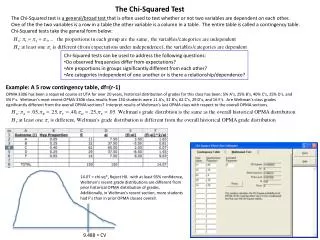
Critical Chi-Squared In our football problem above, we had a chi-squared of 17.68 in a cross classification table with 2 rows and 3 columns. Our chi-squared distribution for that table has df = (2 – 1) * (3 – 1) = 2. According to A.4, with -level = .05, Critical Chi-Squared is: 5.99. Since 17.68 > 5.99, we reject the null. We reject that our sample could have come from a population where sex was not related to attitudes toward football. df = 2 Football Chi-squared 5% of 2 values 2 5.99 17.68
Chi-Squared 7-Step Significance Test Now let’s get formal… 7 steps to Chi-squared test of independence: • Set -level (e.g., .05) • Find Critical 2 (depends on df and -level) • The null and alternative hypotheses: Ho: The two variables are independent of each other Ha: The two variables are dependent on each other • Collect Data • Calculate 2 : 2 = ((fo - fe)2 / fe) • Make decision about the null hypothesis • Report the p-value
Chi-Squared Interpretation Afterwards, what is discovered? If Chi-Squared is not significant, the variables are unrelated. If Chi-Squared is significant, the variables are related. That’s All! Chi-Squared cannot tell you anything like the strength or direction of association. For purely nominal variables, there is no “direction” of association.
Chi-Squared Properties Other points… • Chi-Squared is a large-sample test. If dealing with small samples, look up appropriate tests. (A condition of the test: no expected frequency lower than 5 in each cell) • The larger the sample size, the easier it is for Chi-Squared to be significant. • 2 x 2 table Chi-Square gives same result as Independent Samples t-test for proportion and ANOVA.
Cross Tabs, Strength and Direction of Association - Ordinal Variables Further topics you could explore: Strength of Association • Discussing outcomes in terms of difference of proportions • Reporting Odds Ratios (likelihood of a group giving one answer versus other answers or the group giving an answer relative to other groups giving that answer) • Yule’s Q and Phi: for 2x2 tables, ranging from -1 to 1, with 0 indicating no relationship and 1 a strong relationship Strength and Direction of Association for Ordinal--not nominal--Variables • Gamma (an inferential statistic, so check for significance) Ranges from -1 to +1 Valence indicates direction of relationship Magnitude indicates strength of relationship Chi-squared and Gamma can disagree when there is a nonrandom pattern that has no direction. Chi-squared will catch it, gamma won’t. • Tau c • Kendall’s tau-b • Somer’s d
Cross Tabs and Chi-SquaredControlling for a Third Variable • Controlling for a third variable. • One can see the relationship between two variables for each level of a third variable. • E.g., Sex and Football by Lower or Upper Division. Yes No Maybe Upper F M Yes No Maybe Lower F M
Cross Tabs and Chi-SquaredControlling for a Third Variable • Sex and Pornlaws
Cross Tabs and Chi-SquaredControlling for a Third Variable • Sex and Pornlaw by Sex Education
Cross Tabs and Chi SquaredAnother Example • A criminologist is interested in the effects of placement type on recidivism and severity of crime. He collects data from delinquents in four placement types: • Boot Camp (n = 50) • Wilderness Expedition (n = 75) • Electronic Supervision (n = 100) • Residential Treatment (n = 25) • He records records recidivism and severity of crime. The categories are no crime (NC), minor (MI), moderate (MO), serious (S). • Severity for each group includes: NC MI MO S • Boot Camp: 20 15 5 10 • Wilderness Expedition: 30 20 15 10 • Electronic Supervision: 25 35 20 20 • Residential Treatment: 5 5 10 5