Chi Squared Tests
Chi Squared Tests. Introduction. Two statistical techniques are presented. Both are used to analyze nominal data. A goodness-of-fit test for a multinomial experiment. A contingency table test of independence. The test statistics in both cases follow the c 2 distribution.


Chi Squared Tests
E N D
Presentation Transcript
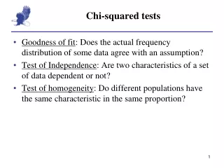
Introduction • Two statistical techniques are presented. Both are used to analyze nominal data. • A goodness-of-fit test for a multinomial experiment. • A contingency table test of independence. • The test statistics in both cases follow the c2 distribution.
Chi-Squared Goodness-of-Fit Test • The hypothesis tested involves the “success” probabilities p1, p2, …, pk.of a multinomial distribution. • The multinomial experiment is an extension of the binomial experiment. • There are n independent trials. • The outcome of each trial can be classified into one of k categories, called cells. • The probability pi for an outcome to fall into cell i remains constant for each trial. By assumption, p1 + p2 + … +pk = 1. • Trials in the experiment are independent.
Our objective is to find out whether there is sufficient evidence to reject a pre-specified set of values for pi . • The hypotheses: • The test builds on comparing actual frequency and the expected frequency of occurrences in all cells.
An Example • Example 16.1 • Two competing companies A and B have been dominant players in the market. Both companies conducted recent advertising campaigns on their products. • Market shares before the campaigns were: • Company A = 45% • Company B = 40% • Other competitors = 15%.
Example 16.1 – continued • To study the effect of the campaigns on the market shares, a survey was conducted. • 200 customers were asked to indicate their preference regarding the products advertised. • Survey results: • 102 customers preferred the company A’s product, • 82 customers preferred the company B’s product, • 16 customers preferred the competitors product.
Example 16.1 – continuedCan we conclude at 5% significance level that the market shares were affected by the advertising campaigns?
Solution • The population investigated is the brand preferences. • The data are nominal (A, B, or other) • This is a multinomial experiment (three categories). • The question of interest: Are p1, p2, and p3 different after the campaign from their values prior to the campaigns?
The hypotheses are: H0: p1 = .45, p2 = .40, p3 =.15 H1: At least one pi changed. The expected frequency for each category (cell) if the null hypothesis is true is shown below: What actual frequencies did the sample return? 90 = 200(.45) 80 = 200(.40) 102 82 30 = 200(.15) 16
The statistic is: Intuitively, this measures the extent of differences between the observed and the expected frequencies. • The rejection region is:
c2 with 2 degrees of freedom • Example 16.1 – continued Alpha P value 5.99 8.18 Rejection region Conclusion: Since 8.18 > 5.99, there is sufficient evidence at 5% significance level to reject the null hypothesis. At least one of the probabilities pi is different. Thus, at least two market shares have changed.
Required Conditions – The Rule of Five • The test statistic used to perform the test is only approximately Chi-squared distributed. • For the approximation to apply, the expected cell frequency has to be at least 5 for all cells (npi³ 5). • If the expected frequency in a cell is less than 5, combine it with other cells.
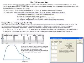
Chi-squared Test of a Contingency Table • This test is used to test whether… • two nominal variables are related? • there are differences between two or more populations of a nominal variable? • To accomplish the test objectives, we need to classify the data according to two different criteria. • The idea is also based on goodness of fit.
Example 16.2 • In an effort to better predict the demand for courses offered by a certain MBA program, it was hypothesized that students’ academic background affect their choice of MBA major, thus, their courses selection. • A random sample of last year’s MBA students was selected. The following contingency table summarizes relevant data.
If each classification is considered a nominal variable, are these two variables dependent? If each undergraduate degree is considered a population, do these populations differ? The observed values There are two ways to view this problem
The test statistic • The rejection region k is the number of cells in the contingency table. Since ei = npi but pi is unknown, we need to estimate the unknown probability from the data, assuming H0 is true. • Solution • The hypotheses are: H0: The two variables are independent H1: The two variables are dependent
Estimating the expected frequencies Undergraduate MBA Major Degree Accounting Finance Marketing Probability 60 BA 60 60/152 BENG 31 31/152 39 BBA 39 39/152 Other 22 22/152 152 61 44 152 61 44 47 152 Probability 61/152 44/152 47/152 Under the null hypothesis the two variables are independent: P(Accounting and BA) = P(Accounting)*P(BA) = [61/152][60/152]. The number of students expected to fall in the cell “Accounting - BA” is eAcct-BA = n(pAcct-BA) = 152(61/152)(60/152) = [61*60]/152 = 24.08 The number of students expected to fall in the cell “Finance - BBA” is eFinance-BBA = npFinance-BBA = 152(44/152)(39/152) = [44*39]/152 = 11.29
(Column j total)(Row i total) Sample size eij = • The expected frequency of cell of row i and column j in the contingency table is calculated by:
Calculation of the c2 statistic • Solution – continued Undergraduate MBA Major Degree Accounting Finance Marketing 31 24.08 BA 31 (24.08) 13 (17.37) 16 (18.55) 60 BENG 8 (12.44) 16 (8.97) 7 (9.58) 31 31 24.08 BBA 12 (15.65) 10 (11.29) 17 (12.06) 39 7 6.80 5 6.39 Other 10 (8.83) 5 (6.39) 7 (6.80) 22 31 24.08 61 44 47 152 7 6.80 5 6.39 31 24.08 The expected frequency 7 6.80 5 6.39 31 24.08 7 6.80 5 6.39 (31 - 24.08)2 24.08 c2= (5 - 6.39)2 6.39 (7 - 6.80)2 6.80 = 14.70 +….+ +….+
Solution – continued • The critical value in our example is: • Conclusion: • Since c2 = 14.70 > 12.5916, there is sufficient evidence to infer at 5% significance level that students’ undergraduate degree and MBA students courses selection are dependent.
Using the computer Select the Chi squared / raw data Option from Data Analysis Plus under tools. See Xm16-02 Define a code to specify each nominal value. Input the data in columns one column for each category. Code: Undergraduate degree 1 = BA 2 = BENG 3 = BBA 4 = OTHERS MBA Major 1 = ACCOUNTING 2 = FINANCE 3 = MARKETING