Download
1 / 21
210 likes | 237 Views
Chi-Squared tests ( 2 ) :. score per participant ( aim for this, where possible). categorical data ( avoid this, where possible). "psycho". "non-psycho". Chi-Squared tests ( 2 ) :

E N D
score per participant (aim for this, where possible) categorical data (avoid this, where possible) "psycho" "non-psycho" Chi-Squared tests (2): Use with nominal (categorical) data – when all you have is the frequency with which certain events have occurred.
The 2 “Goodness of Fit” test: Compares an observed frequency distribution with an expected frequency distribution. Useful when you have the observed frequencies for a number of mutually- exclusive categories, and you want to decide if they have occurred equally frequently.
Which soap-powder name do shoppers like best? Each of 100 shoppers picks the powder name they like most. Number of shoppers picking each name (observed frequencies): Washo Scruba Musty Stainzoff Beeo total 40 35 5 10 10 100 Expected frequency for each category is total no.observations / number of categories 100 / 5 = 20.
The formula for Chi-Square: Washo Scruba Musty Stainzoff Beeo total O: 40 35 5 10 10 100 E: 20 20 20 20 20 100 (O-E): 20 15 -15 -10 -10 (O-E) 2 400 225 225 100 100 20 11.25 11.25 5 5 2 = 52.5
Chi-squared is the sum of the squared differences between each observed frequency and its associated expected frequency. The bigger the value of 2, the greater the difference between observed and expected frequencies. But how big does 2 have to be, to be regarded as “big”? Is 52.5 “big”?
We compare our obtained2 value to 2 values which would be obtained by chance. To do this, we need the “degrees of freedom”: this is the number of categories (or “cells”) minus one. We have a 2 value of 52.5, with 5-1 = 4 d.f. Tables show how likely various values of 2 are to occur by chance. e.g.: probability level: d.f. .05 .01 .001 1 3.84 6.63 10.83 2 5.99 9.21 13.82 3 7.81 11.34 16.27 4 9.49 13.28 18.46 5 11.07 etc. etc. 52.5 is bigger than 18.46, a value of 2 which will occur by chance less than 1 times in a 1000 (p<.001).
With 4 d.f., 2 values of 9.49 or more are likely to occur by chance on less than .05 of occasions. The sampling distribution of chi-square: Frequency with which 2 values occur purely by chance:
Our obtained 2 = 52.5, with 4 d.f., p < .001. A 2 value this large is highly unlikely to have arisen by chance. It appears that the distribution of shoppers’ choices across soap-powder names is not random. Some names get picked more than we would expect by chance and some get picked less.
The 2 test of association between two independent variables: Another common use of 2 is to determine whether there is an association between two independent variables. Is there an association between gender (male or female: IV A) and soap powder (Washo, Musty, etc.: IV B)?
This gives a 2 x 5 contingency table. Data for a random sample of 100 shoppers, 70 men and 30 women: Washoe Scrubbup Musty Stainoff Nogunge total male 10 12 5 3 40 70 female 6 2 1 20 1 30 totals: 16 14 6 23 41 100
To calculate expected frequencies: E = row total * column total grand total Work out the expected frequency for each cell: e.g. 11.2 = (16 * 70)/100 6.9 = (23 * 30)/100, etc.
Using exactly the same formula as before, we get 2 = 52.94. d.f. = (number of rows - 1) * (number of columns - 1). We have two rows and five columns, so d.f. = (2-1) * (5-1) = 4 d.f. Use the same table to assess the chances of obtaining a Chi-Squared value as large as this by chance; again p< .001. Conclusion: our observed frequencies are significantly different from the frequencies we would expect to obtain if there were no association between the two variables: i.e. the pattern of name preferences is different for men and women.
Chi-Square test merely tells you that there is some relationship (an association) between the two variables in question: it does not tell you anything about the causal relationship between the two variables. Here, it is reasonable to assume that gender causes people to pick different soap powder names; it's unlikely that soap powder names cause people to be male or female. However, in principle the direction of causality could equally well go in either direction.
Assumptions of the Chi-Square test: 1. Observations must be independent: each subject must contribute to one and only one category. Otherwise the test results are completely invalid. 2. Problems arise when expected frequencies are very small. Chi-Square should not be used if more than 20% of the expected frequencies have a value of less than 5. (It does not matter what the observed frequencies are). Two solutions: combine some categories (if this is meaningful in your experiment), OR obtain more data (make the sample size bigger).
2 test of association - the one- d.f. case: Preferred TV programme: Stenders: Corrie: Row total: Origin: North: 13 10 23 South: 5 24 29 Column total: 18 34 52 With 1 d.f. (as with a 2 x 2 table), the obtained 2 value is inflated; some statisticians advocate using "Yates' Correction for Continuity" to make the 2 test more conservative (i.e. make 2 value smaller and hence less likely to be significant).
Same procedure as before, except (a) take the absolute value of O - E (i.e., ignore any negative signs). (b) Subtract 0.5 from each O-E, before squaring it. Without Yates’ Correction: 2 = 8.74. With Yates’ Correction: 2 = 7.09.
Why you should avoid using Chi-Square if you can: Design studies so that you can avoid using Chi-Square! Frequency data give little information about participants' performance: all you have is knowledge about which category someone is in, a very crude measure. It's much more informative to obtain one or more scores per participant; scores give you more information about performance than categorical data (and can be used with better statistical tests). e.g. IQ: which is better - to know participants are “bright” or “dim”, or have their actual IQ scores?
2 Goodness of Fit test on "fast food" data, using SPSS: Are all brands mentioned equally frequently? Analyze > Nonparametric Tests> Legacy Dialogs > Chi-Square
2 test of association on "fast food" data, using SPSS: Is there an association between gender and brand first mentioned? Analyze > Descriptive Statistics > Crosstabs...
2 test of association on "fast food" data (continued): Is there an association between gender and brand first mentioned? 11 response categories - gives too many expected frequencies < 5. Therefore confined analysis to Burger King, KFC and McDonalds. (Use "Select Cases" on "Data" menu to filter out unwanted response categories). Conclusion: no significant association between gender and brand first mentioned. (2 (2) = 0.28, p = .87)