EXAMINING RELATIONSHIPS
This guide explores Least Squares Regression (LSR), a statistical method used to find the best-fitting straight line through a set of data points. We discuss how a regression line predicts the response variable (y) using an explanatory variable (x), the significance of slope and intercept in interpreting data, and the mathematical formulation of LSR. Through practical examples, including predicting natural gas consumption based on temperature, we illustrate how LSR minimizes prediction errors and enhances data analysis.

EXAMINING RELATIONSHIPS
E N D
Presentation Transcript
EXAMINING RELATIONSHIPS Least Squares Regression
Least Squares Regression • A regression line is a straight line that describes how a response variable y changes as an explanatory variable x changes. • The least squares regression line (LSRL) is a mathematical model for the data. • We often use a regression line to predict the value of y for a given value of x. • Regression, unlike correlation, requires that we have an explanatory variable and a response variable.
Least Squares Regression • A regression line is a straight line that describes how a response variable y changes as an explanatory variable x changes. • The least squares regression line (LSRL) is a mathematical model for the data. • We often use a regression line to predict the value of y for a given value of x. • Regression, unlike correlation, requires that we have an explanatory variable and a response variable.
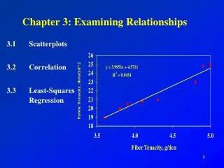
Least Squares Regression • Example 3.9 • On the next slide is the least squares regression line of Figure 3.2. • We can use this line to predict the natural gas consumption for this family. • For example, “If a month averages 20 degree days per day (45ºF), how much gas will the family use?” • Locate 20 on the x-axis, then go up and over to find the consumption on the y-axis that corresponds to x=20. • The family will use about 4.9 hundreds of cubic feet of gas each day.
Least Squares Regression • Investigating the least squares regression line • Different people might draw different lines by eye on a scatterplot, especially when the points are widely scattered. • We want a line that can be used to predict y from x
Least Squares Regression • Investigating the least squares regression line • We also want a line that is as close as possible in the vertical direction to each point. • Prediction errors occur in y, that is why we want a line as close as possible in the vertical direction. • When we made the prediction that the family would use 4.9 hundreds of cubic feet for a month with 20 degree days it is possible that the prediction has some error involved in it. • For example if the actual usage turns out to be 5.1 hundreds of cubic feet we have an error of .2
Least Squares Regression • Investigating the least squares regression line • We want a regression line that makes the vertical distance from each point on the scatterplot as small as possible. • In figure 3.10a (see the next slide) there are three points from figure 3.9 along with the line on an expanded scale. • The line passes above two of the points and below one of them • The vertical distances of the data points appear as vertical line segments.
Least Squares Regression • One reason the LSRL is so popular is that the problem of finding the line has a simple answer. • We can give the recipe for the LSRL in terms of the means and the standard deviations of the two variables and their correlation.
Least Squares Regression • EQUATION OF THE LEAST SQUAES REGRESSION LINE • We have data on an explanatory variable x and a response variable y for n individuals. From the data, calculate the means and the standard deviations of the two variables, and their correlation r. • The LSRL is the line with slope b and y-intercept a. p. 150 3.36a, b
Least Squares Regression • We write (read “y hat”) in the equation of the regression line to emphasize that the line is a predicted response for any x. • The predicted response will usually not be exactly the same as the actually observed response y.
Least Squares Regression • The least squares regression line as reported by the TI83 calculator is • Do not forget to put the hat symbol over the y to show the predicted value.
Least Squares Regression • Slope • Slope of a regression line is usually important for the interpretation of the data. • The slope is the rate of change, the amount of change in y when x increases by 1. • The slope in this example is .1890. Meaning that on the average, each additional degree day predicts consumption of .1890 more hundreds of cubic feet of natural gas per day.
Least Squares Regression • Intercept • The intercept of a line is the value of y when x=0. • In our example, x=0 when the average outdoor temperature is at least 65ºF. • Substituting x=0 into the least squares regression line gives a y-intercepts of 1.0892 hundreds of cubic feet of gas per day when there are no degree days.
Least Squares Regression • Predicting • The least squares regression line makes predicting easy. • To predict gas consumption at 20 degree days, substitute x=20 to get a y=4.869.
Least Squares Regression • The least squares regression line makes predicting easy. • To predict gas consumption at 20 degree days, substitute x=20 to get a y=4.869.
Least Squares Regression • Plotting the line • To plot the line, use the equation to find y for two values of x • One value should be near the lower end of the range of x and one value should be at the high end. • Plot each y above its x and draw the line
Least Squares Regression • Least squares regression line with the actual data and the two points from the least squares regression equation.
Least Squares Regression p. 142 3.31, 3.33 Together p. 161 3.42 – 3.45, 3.47, 3.48
Least Squares Regression • Facts about least-squares regression • Example 3.11 • Figure 3.11(see next slide) shows a scatterplot that played a central role in the discovery that the universe is expanding. • The data represents the distances from the earth of 24 galaxies and the speed at which these galaxies are moving away from us reported by the astronomer Edwin Hubble in 1929.
Least Squares Regression • Facts about least-squares regression • Example 3.11 • This relationship is a linear relationship with a correlation r=.7892 • This relationship shows that more distant galaxies are moving away more rapidly. • It is important to note that astronomers now believe that this relationship is in fact a perfect relationship, and that the scatter is caused by imperfect measurements.
Least Squares Regression • Facts about least-squares regression • Example 3.11 • The two lines on the plot are the two least squares regression lines. • The regression line of velocity on distance is solid. • The regression line of distance on velocity is dashed. • Regression of velocity on distance and regression of distance on velocity give different lines. • Remember to make sure you know which variable is explanatory
Least Squares Regression • Facts about least-squares regression • Even though correlation, r, ignores the distinction between explanatory and response variables, there is a close connection between correlation and regression. • The slope(b) of the least squares regression line means that a change of one standard deviation in x corresponds to a change of r standard deviations in y. • The slope(b) of the least squares regression line means that a change of one standard deviation in x corresponds to a change of r standard deviations in y.
Least Squares Regression • Facts about least-squares regression • SLOPE OF THE LEAST SQUARES REGRESSION LINE • When the variables are perfectly correlated, that is r=1 or r=-1, the change in the predicted response y is the same as the change in x. • When , the change in y is less than the change in x. • Meaning that as the correlation grows less strong, the prediction y moves less in response to changes in x.
Least Squares Regression • The coefficient of determination, r2, is the number we use to determine how well x predicts y • Facts about least-squares regression • One way to determine the usefulness of the least squares regression model is to measure how well x predicts y.
Least Squares Regression • Facts about least-squares regression • If x is a good predictor of y, then the r2 will be close to 1 or 100% • Therefore there is an 84% chance that the predicted value is correct • We can then say that x is a pretty good predictor of y
Least Squares Regression • Facts about least-squares regression • If x is a poor predictor of y, then r2 will be close to 0 0% • Therefore there is an 3.57% chance that the predicted value is correct • We say that 3.57% of the variation in y is explained by least squares regression of y on x. • We can now say that x is not a good predictor of y
Least Squares Regression • Facts about least-squares regression • When you report a regression, give r2 as a measure of how successful the regression was in explaining the response. • When you see a correlation, square it to get a better feel for the strength of the association. • Perfect correlations mean the points lie exactly on a line. Then r2=1 and thus, x will always predict y.
Least Squares Regression • Facts about least-squares regression • If r=-.7 or r=.7, then r2=.49 and about half the variation is accounted for by the linear relationship. • In the r2 scale, correlation of ±.7(r), is about halfway between 0 and ±1(r2). • The special properties of least squares regression is another reason why it is the most common method of fitting a regression line to data.
Least Squares Regression • P. 150 3.36c, 3.37, 3.38 Together
Least Squares Regression • RESIDUALS • A residual is the difference between an observed value of the response variable and the value predicted by the regression line. • That is residual = observed y – predicted y • Pay attention to your window on your calculator when looking at a residual plot
Least Squares Regression • RESIDUALS • Example 3.15 • Does the age at which a child begins to talk predict a later score on a test of mental ability? • A study of the development of young children recorded the age in months at which each of the 21 children spoke their first word and Gesell Adaptive Test Score (an aptitude test taken much later) • The data appear in Table 3.4 • The scatterplot with age at first word as the explanatory vairable x and Gesell score as the response variable y appears in Figure 3.14.
Least Squares Regression • RESIDUALS
Least Squares Regression • RESIDUALS • Example 3.15 Continued • Children 3 and 13 and also children 16 and 21 are marked with a different plotting symbol because they have identical values of both variables. • The plot shows that children who begin to speak later tend to have lower test scores than early talkers (negative association). • The overall pattern is moderately linear with a correlation of r=-.640
Least Squares Regression • Example 3.15 Continued • RESIDUALS • The regression line is • For child 1, who first spoke at 15 months, the predicted score would be 92.97 • The actual score was 95. • So the residual is 95-92.97=2.03 • The residual is positive because the data point lies above the line.
Least Squares Regression • Example 3.15 Continued • RESIDUALS • There is a residual for each data point • Here are the 21 residuals for the data (TI83 or Microsoft Excel)
Least Squares Regression • Example 3.15 Continued • RESIDUALS • Check the residuals to see how well the regression line fits the data. • Look at the vertical deviations of the points from the line in a scatterplot of the original data (Figure 3.14.) • A residual plot, plots the residuals on the vertical axis against the explanatory variable (Figure 3.15) • This makes the patterns easier to see. • Residuals from least squares regression always have a mean of zero. • When you check the sum of the 21 residuals you get -.0002 because the numbers were rounded (roundoff error)
Least Squares Regression • What should a residual plot look like • RESIDUALS • The ideal pattern for a residual plot is Figure 3.16a. • The plot shows a uniform scatter of points above and below the fitted line • The plot shows no unusual individual observations
Least Squares Regression • Examining Residuals • RESIDUALS • A curved pattern is not a good model for such data (Figure 3.16B on the next slide) . • Increasing or decreasing spread about the line as x increases produces a prediction of y that will be less accurate for larger values of x in that example (Figure 3.16c on the next slide). • Individual points with large residuals like child 19 in Figures 3.14 and 3.15 are outliers because they are outside the straight line pattern. • Individual points that are extreme in the x direction, like Child 18 in Figures 3.14 and 3.15, but do not have large residuals can be very important.
Least Squares Regression • In the Gesell Test Scores example, Child 18 and Child 19 are unusual in their own way. • Individual Observations • Child 19 lies far from the regression line, where as Child 18 lies close to the line but far out in the x direction. • Child 19 is an outlier, with Gesell score so high that we should check for a mistake in recording. • Child 18 began to speak much later than any of the other children • Because of the extreme position on the age scale, this point has a strong influence on the position of the regression line.
Least Squares Regression • Figure 3.17 (next slide) adds a second regression line, calculated after leaving out Child 18. • Individual Observations • You can see that this one point moves line quite a bit. • Least squares regression lines make the sum of squares of the vertical distances to the points as small as possible. • A point that is extreme in the x direction with no other points near it pulls the line toward itself (influential).
Least Squares Regression • An outlier is an observation that lies outside the overall pattern of the other observations in a scatterplot. • Individual Observations • An observation can be an outlier in the x direction, in the y direction, or in both directions. • An observation is influential if removing it would markedly change the position of the regression line. • Points that are outliers in the x direction are often influential.
Least Squares Regression • Child 18 is an outlier in the x direction and is influential. • Individual Observations • Child 19 is an outlier in the y direction but has less influence on the regression line because there are many of the other points with similar values of x that anchor the line well below the outlying point. • Influential points often have small residuals, because they pull the line toward themselves. • You must do more than just look at the residuals to find influential points.