Download
1 / 43
430 likes | 586 Views
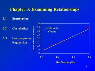
Chapter 3: Examining Relationships . 3.1 Scatterplots 3.2 Correlation 3.3 Least-Squares Regression. Relationship Between Fiber Tenacity and Fabric Tenacity. Variable Designations. Which variable is the dependent variable ? Our text uses the term response variable .

E N D
Chapter 3: Examining Relationships 3.1 Scatterplots 3.2 Correlation 3.3 Least-Squares Regression
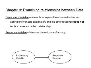
Variable Designations • Which variable is the dependent variable? • Our text uses the term response variable. • Which variable is the independent variable? • Explanatory variable • Note: Sometimes we do not have a clear explanatory-response variable situation … we may just want to look at the relationship between two variables. • Problems 3.1 and 3.4, p. 123
Scatterplot 1: Relationship Between FiberTenacity and Fabric Tenacity Note placement of response and explanatory variables. Also note axes labels and plot title.
Problem 3.6, p. 125 • Type data into your calculator. • Examining a scatterplot: • Look for the overall pattern and striking deviations from that pattern. • Pay particular attention to outliers • Look at form, direction, and strength of the relationship.
Examining a Scatterplot, cont. • Form • Does the relationship appear to be linear? • Direction • Positively or negatively associated? • Strength of Relationship • How closely do the points follow a clear form? • In the next section, we will discuss the correlation coefficient as a numerical measure of strength of relationship.
Tips for Drawing Scatterplots • p. 128
Homework • Reading: pp. 121-135
Practice • Problems: • 3.11 (p. 129) • 3.12 (p. 132) • 3.16 (p. 136)
The two plots represent the same data! • Our eye is not good enough in describing strength of relationship. • We need a method for quantifying the relationship between two variables. • The most common measure of relationship is the Pearson Product Moment correlation coefficient. • We generally just say “correlation coefficient.”
Correlation Coefficient, r • The correlation, r, is an average of the products of the standardized x-values and the standardized y-values for each pair.
Correlation Coefficient, r • A correlation coefficient measures these characteristics of the linear relationship between two variables, x and y. • Direction of the relationship • Positive or negative • Degree of the relationship: How well do the data fit the linear form being considered? • Correlation of (1 or -1) represents a perfect fit. • Correlation of (0) indicates no relationship.
Interpreting Correlation Coefficient, r • Correlation Applet: http://www.duxbury.com/authors/mcclellandg/tiein/johnson/correlation.htm • Facts about correlation • pp.143-144 • Correlation is not a complete description of two-variable data. We also need to report a complete numerical summary (means and standard deviations, 5-number summary) of both x and y.
Outlier, or influential point? • Let’s enter the data into our calculators and calculate the correlation coefficient. The data are in the middle two columns of Table 1.10, p. 59. • r=? • Now, remove the possible influential point. What happens to r?
Exercises: Understanding Correlation • Review “Facts about correlation,” pp. 143-144 • 3.34, 3.35, and 3.37, p. 149 • Reading: pp. 149-157
Least Squares Regression • Ultimately, we would like to predict elongation by using a more practical measurement, winding tension. • A regression line, also called a line of best fit, was found. • How was the line of best fit determined? • Determine mathematically the distance between the line and each data point for all values of x. • The distance between the predicted value and the actual (y) value is called a residual (or error).
Least Squares Regression: Line of Best Fit • This could be done for each data point. If we square each residual and sum all of the squared residuals, we have: • The best-fitting line is the line that has the smallest sum of e2 ... the least squares regression line! That is, the line of best fit occurs when:
Least-Squares Regression Line • With the help of algebra and a little calculus, it can be shown that this occurs when:
Exercise 3.12, p. 132 • Is there a relationship between lean body mass and resting metabolic rate for females? • Quantify this relationship. • Find the line of best fit (the least-squares regression, LSR). • Use the LSR to predict the resting metabolic rate for a woman with mass of 45 kg and for a woman with mass of 59.5 kg.
Interpreting the Regression Model • The slope of the regression line is important for the interpretation of the data: • The slope is the rate of change of the response variable with a one unit change in the explanatory variable. • The intercept is the value of y-predicted when x=0. It is statistically meaningful only when x can actually take values close to zero.
R2: Coefficient of Determination • Proportion of variability in one variable that can be associated with (or predicted by) the variability of the other variable. 1- r2 = 0.28 r = 0.85, r2 = 0.72
Residuals • In regression, we see deviations by looking at the scatter of points about the regression line. The vertical distances from the points to the least-squares regression line are as small as possible, in the sense that they have the smallest possible sum of squares. • Because they represent “left-over” variation in the response after fitting the regression line, these distances are called residuals.
Examining the Residuals • The residuals show how far the data fall from our regression line, so examining the residuals helps us to assess how well the line describes the data. • Residuals Plot
Residuals Plot • Let’s construct a residuals plot, that is, a plot of the explanatory variable vs. the residuals. • pp. 174-175 • The residuals plot helps us to assess the fit of the least squares regression line. • We are looking for similar spread about the line y=0 (why?) for all levels of the explanatory variable.
Residuals Plot Interpretation, cont. • A curved or other definitive pattern shows an underlying relationship that is not linear. • Figure 3.19(b), p. 170 • Increasing or decreasing spread about the line as x increases indicates that prediction of y will be less accurate for smaller or larger x. • Figure 3.19(c), p. 171 • Look for outliers!
How to create a residuals plot • Create regression model using your calculator. • Create a column in your STAT menu for residuals. Remember that a residual is the actual value minus the predicted value:
HW • Read through end of chapter • Problems: • 3.42 and 3.43 (parts a and b only), p. 165 • 3.46, p. 173 • Chapter 3 Test on Monday
Regression Outliers and Influential Observations • A regression outlier is an observation that lies outside the overall pattern of the other observations. • An observation is influential for a statistical calculation if removing it would markedly change the result of the calculation. • Points that are outliers in the x direction of a scatterplot are often influential for the least-squares regression line. • Sometimes, however, the point is not influential when it falls in line with the remaining data points. • Note: An influential point may be an outlier in terms of x, but we label it as “influential” if removing it significantly influences the regression.
Practice Problems • Problems: • 3.56, p. 179 • 3.74, p. 188 • 3.76, p. 189
Preparing for the Test • Re-read chapter. • Know the terms, big concepts. • Chapter Review, pp. 181-182 • Go back over example and HW problems. • Study slides!