Download
1 / 53
530 likes | 651 Views
This chapter dives into the concepts of scatterplots and correlation, crucial tools for examining relationships between variables in data analysis. It defines the response and explanatory variables, emphasizing the necessity of distinguishing between them. Key techniques for analyzing scatterplots, such as identifying direction, form, and strength of relationships, are outlined. Additionally, it highlights that correlation, while indicating the strength of linear relationships, does not imply causation and is sensitive to outliers. Readers will also learn about Least Squares Regression and its applications in predicting outcomes.

E N D
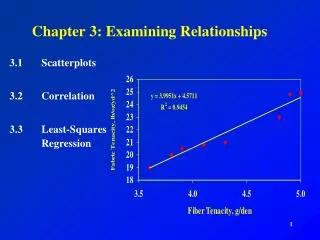
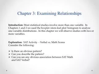
Chapter 3Examining Relationships Section 3.1 Scatterplots
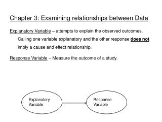
Terms to Know A response variable measures an outcome of a study. An explanatory variable attempts to explain the observed outcomes.
Example of an Explanatory and Response Variable One degree day is accumulated for each degree a day’s average temp falls below or rises above 65 degrees.
Key Concept The statistical techniques used to study relations among variables are more complex than one-variable methods. Fortunately we build on the tools used for examining individual variables. The principles that guide examination are the same. • Start with a graph • Look for an overall pattern and deviations from the pattern • Add numerical descriptions of specific aspects of the data • Sometimes there is a way to describe that
Term to Know The most effective way to display the relation between two quantitative variables is a scatterplot. Plot the explanatory variable, if there is one, on the x-axis, and the response variable on the y-axis. Each individual in the data appears as a point.
Interpreting Scatterplots To interpret a scatterplot, look first for a pattern. The pattern should reveal direction, form and strength of the relationship between two variables. Refer to Figure 3.1 on page 175. Form: two clusters Direction: Negatively associated Strength: moderate
Yes, you can have outliers on ScatterPlots An outlier in any graph of data is an individual observation that falls outside the overall pattern of the graph (ie: WV)
Add a Third Variable (Categorical) of Southern and non-Southern by Using Different Symbols
Scatter Plot Heads Up When several individuals have exactly the same data, they occupy the same point on the scatter plot. Some software packages address the issue by using different symbols for multiple individuals with the same data. You can do the same by hand. However, your calculator does not. So be careful. Use trace to identify such cases.
Scatterplots display direction, form, strength and relationship between two variables. However, our eyes are not a good judge of the strength of the relationship.
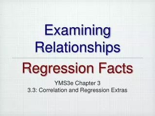
Key Concept Correlation measure the direction and strength of the linear relationship between two quantitative variables. Correlation is usually written as r.
Facts About Correlation • No distinction between explanatory and response variable • Requires two quantitative variables • Unit change of observation does not change correlation • Positive r indicates positive association, negative r indicates negative association • Range: -1 < r < 1 • Measures strength of linear relationships of two variables only • Is not resistant to outliers
Correlation Exercise • Technology Toolbox, page 186 • Yes, The process is long and convoluted, but there is a shortcut using LinReg Command
Key Concept 1) A key thing to remember when working with correlations is never to assume a correlation means that a change in one variable causes a change in another. Sales of personal computers and athletic shoes have both risen strongly in the last several years and there is a high correlation between them, but you cannot assume that buying computers causes people to buy athletic shoes (or vice versa).
Key Concept 2) Correlation only describes linear relationships only, now matter how strong how strong the curved relationship may be. • Like mean and standard deviation, correlation, r, is not resistant to outliers • Correlation is not a complete summary of a two variable relationship. You should give the means of x and y.
Homework • Read 3.2 • Complete problems 1, 2, 6, 7 ,8, 13, 15, 19, 21, 23
Chapter 3Examining Relationships Section 3.2 Least-Squares Regression
Key Term Least Squares Regression is a method for finding a line the summarizes the relationship between two variables that show a linear trend. We often use a regression line to predict the value of y for a given value of x. Regression, unlike correlation requires that we have an explanatory variable and a response variable.
Regression Line for Predicting Gas Consumption from Degree Days
LSRL – Using TI84 Enter NEA data in L1 and Fat data in L2
NEA/Fat Least-Squares Regression Line Exercise Complete Technology Toolbox on page 210
Interpret you regression equation in terms of your variables(ie: fat gain = a + b(NEA change)
Use your Model to predict weight gain given an NEA of 400 (interpolation) Use your Model to predict weight gain given an NEA of 1000 (extrapolation)
Equation of the Least-Squares Regression Line • You can manually calculate the equation of the Least-Squares Regression Line With slope And Intercept
Homework • Exercises 3.29 – 32, 35, 36 • Read Section 3.3
Chapter 3Examining Relationships Section 3.2 Least-Squares Regression (Continued) Section 3.3 Correlation and Regression Wisdom
Key Concept • A residual is the difference between and observed value of the response variable and the value predicted by the regression line. That is, residual = observed y – predicted y
Interpreting a Residual Plot • The uniform scatter of points indicates the regression line fits the data well, so the line is a good model.
Interpreting a Residual Plot • The residual have a curved pattern, so a straight line is an inappropriate model
Interpreting a Residual Plot • The response variable y has more spread for larger values of the explanatory variable x, so prediction will be less accurate when x is large.
Create a Residual Plot with Hand-Span Data Follow procedures detailed in Technology toolbox on page 219
Key Concept The coefficient of determination, r2, is the fraction of the variation in the values of y that is explained by least-squares regression of y on x. Eg: ____% of the variation in Height is accounted for by the linear relationship between hand size and Height.
Facts about Least-Squares Regression • Fact 1 – The distinction between explanatory and response variables is essential in regression
Facts about Least-Squares Regression • Fact 2 – There is a close connection between correlation and the slope of the least squares line. The slope is:
Facts about Least-Squares Regression • Fact 3 – The least squares line always passes through the point
Constructing the Least-Squares Example Suppose we have explanatory and response variables and we know that the mean of x=17, mean of y=161.111, sx=19.696, sy=33.479 and the correlation r = .997. Even though we don’t know the actual data, we can still construct the equation for the least-squares line and use it to make predictions.
Constructing the Least-Squares Example So the Least-squares Line has an equation
Facts about Least-Squares Regression • Fact 4 – The correlation r describes the strength of a straight-line relationship. In the regression setting, this description takes a specific form: The square of the correlation, r2 , is the fraction of the variation in the values of y that is explained by the least-squares regression of y on x.
Key Concept • Correlation and regression describe only linear relationships • Extrapolation (using a model outside of the range of the data) often produces unreliable predictions
Outliers and Influential Observations in Regression • An outlier is an observation that lies outside the overall pattern of the other observations • An observation is influential for a statistical calculation if removing it would markedly change the result of the calculation. Points that are outliers in the x direction of a scatter plot are often influential for the least-squares regression line. (Example: Revisit correlation applet)
Child 19 and Child 18 are both outliers. Child 18 is more influential.