Examining Relationships
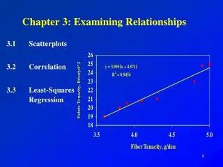
Examining Relationships. Regression Facts. YMS3e Chapter 3 3.3: Correlation and Regression Extras. Regression Basics. When describing a Bivariate Relationship: Make a Scatterplot Strength, Direction, Form Model: y-hat=a+bx Interpret slope in context Make Predictions

Examining Relationships
E N D
Presentation Transcript
Examining Relationships Regression Facts • YMS3e Chapter 3 • 3.3: Correlation and Regression Extras
Regression Basics • When describing a Bivariate Relationship: • Make a Scatterplot • Strength, Direction, Form • Model: y-hat=a+bx • Interpret slope in context • Make Predictions • Residual = Observed-Predicted • Assess the Model • Interpret “r” • Residual Plot
Minitab Output • Regression equations aren’t always as easy to spot as they are on your TI-84. Can you find the slope and intercept above?
Influential? Outliers/Influential Points • Does the age of a child’s first word predict his/her mental ability? Consider the following data on (age of first word, Gesell Adaptive Score) for 21 children. Does the highlighted point markedly affect the equation of the LSRL? If so, it is “influential”. Test by removing the point and finding the new LSRL.
Explanatory vs. Response • The Distinction Between Explanatory and Response variables is essential in regression. • Switching the distinction results in a different least-squares regression line. • Note: The correlation value, r, does NOT depend on the distinction between Explanatory and Response.
Correlation • The correlation, r, describes the strength of the straight-line relationship between x and y. • Ex: There is a strong, positive, LINEAR relationship between # of beers and BAC. • There is a weak, positive, linear relationship between x and y. However, there is a strong nonlinear relationship. • r measures the strength of linearity...
Coefficient of Determination • The coefficient of determination, r2, describes the percent of variability in y that is explained by the linear regression on x. • 71% of the variability in death rates due to heart disease can be explained by the LSRL on alcohol consumption. • That is, alcohol consumption provides us with a fairly good prediction of death rate due to heart disease, but other factors contribute to this rate, so our prediction will be off somewhat.
Cautions • Correlation and Regression are NOT RESISTANT to outliers and Influential Points! • Correlations based on “averaged data” tend to be higher than correlations based on all raw data. • Extrapolating beyond the observed data can result in predictions that are unreliable.
Correlation vs. Causation • Consider the following historical data: • There is an almost perfect linear relationship between x and y. (r=0.999997) • x = # Methodist Ministers in New England • y = # of Barrels of Rum Imported to Boston • CORRELATION DOES NOT IMPLY CAUSATION!