Download
1 / 99
1.04k likes | 1.22k Views
Gain insights into the Global Forecast System (GFS) by Shrinivas Moorthi. Explore the operational model, initialization methods, vertical and horizontal dynamics, and more for accurate weather predictions.

E N D
Global Forecast System (GFS) Shrinivas Moorthi
What is GFS? Global Forecast System (GFS) is often mislabeled or misunderstood. Global Forecast System is the full global scale numerical weather prediction system – It includes both the global analysis and forecast components However, the term GFS has also been used to imply that it is the NCEP global spectral model. Therefore, we may use the term GFS to imply both the atmospheric model as well as the whole forecast system Shrinivas Moorthi
From the beginning, I would like to make it clear that this presentation is an unpolished mix of slides prepared by various developers of different aspects of the GFS. I have not had the opportunity of going over every slide and make sure that information content is completely correct. Also, I may not be able to correctly interpret individual authors intent while making the slides. There are lots of information in these slides, some are more detailed and some less. For a deeper understanding, I urge you to read the original references and the papers published by the developers, if any, and finally by looking at the code itself. (Also check NCEP website or simply google). Developing these schemes and codes involves lots of engineering and not everything may have complete logical explanation. No attempt is made here to be complete; I spent last one month making sure the system we are installing here works. Shrinivas Moorthi
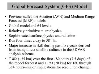
NCEP operational Global Spectral model Horizontal Representation • Spectral (spherical harmonic basis functions) with transformation to a Gaussian grid for calculation of nonlinear quantities and physics • Horizontal resolution • > Operational version - T574 up to 192 hours and T190 to 384 hours • > Supported resolutions – T574, T382, T254, T190, T170, T126 and T62 Shrinivas Moorthi
Initialization • Digital filter initialization with 3 hour window. Time integration scheme: • Leapfrog for nonlinear advection terms • Semi-implicit for gravity waves and zonal advection of vorticity and specific humidity. • Asselin (1972) time filter to control computational mode • Time split physics adjustments with implicit treatment when possible Shrinivas Moorthi
Vertical Domain • Sigma-Pressure hybrid coordinate system • Terrain following near the lower boundary • Constant pressure surfaces in the stratosphere and beyond • Operationally 64 hybrid layers (15 levels below ~ 800 hPa and 24 levels above 100hPa. • 28, 42 and 91 layer options available. Shrinivas Moorthi
Model Dynamics • Prognostic equations • Primitive equations in hybrid sigma-pressure vertical coordinates for vorticity, divergence, (or U,V), ln(Ps), virtual temperature, and tracers. • Tracers can be specific humidity, ozone mixing ratio and cloud condensate mixing ratio or any other aerosol/dust etc. • Operationally only three tracers. • Please see NCEP Office notes #461, 462 for details on equations and numerics Shrinivas Moorthi
Vertical Advection Until the last GFS implementation, the vertical advection of tracers were based on centered difference scheme This resulted in computationally generated negative tracers In the last implementation a positive-definite tracer transport scheme was implemented which minimized the generation of negative tracers. (Fanglin Yang) This change was necessary for the newly implemented GSI which is sensitive to the negative water vapor. Shrinivas Moorthi
Vertical Advection of Tracers: previous GFS Scheme Flux form conserves mass Current GFS uses central differencing in space and leap-frog in time. The scheme is not positive definiteand may produce negative tracers. Shrinivas Moorthi
Vertical Advection of Tracers: Flux-Limited Scheme Thuburn (1993) Van Leer (1974) Limiter, anti-diffusive term Special boundary conditions Shrinivas Moorthi
Vertical Advection of Tracers: Flux-Limited Scheme Thuburn (1993) Van Leer (1974) Limiter, anti-diffusive term Special boundary condition Shrinivas Moorthi
Sources of Negative Water Vapor DataVertical advection assimilation Spectral transform Borrowing by cloud water SAS Convection Example: Removal of Negative Water Vapor _ Ops GFS Data Assimilation Flux-Limited Vertically-Filtered Scheme,central in time Data Assimilation New B: horizontal advection, computed in spectral form with central differencing in space A: vertical advection, computed in finite-difference form with flux-limited positive-definite scheme in space Positive-definite Shrinivas Moorthi Fanglin Yang et al., 2009: On the Negative Water Vapor in the NCEP GFS: Sources and Solution. 23rd Conference on Weather Analysis and Forecasting/19th Conference on Numerical Weather Prediction, 1-5 June 2009, Omaha, NE
Vertical Advection of Tracers: Idealized Case Study wind Upwind (diffusive) Flux-Limited Initial condition GFS Central-in-Space Shrinivas Moorthi
Summary: Negative Water Vapor in the GFS Shrinivas Moorthi
Horizontal Diffusion • Scale selective 8th order diffusion of Divergence, vorticity, virtual, temperature, specific humidity, ozone and cloud condensate. • Temperature diffusion in done on quasi-pressure surfaces Shrinivas Moorthi
Algorithm of the Spectral ModelMike Young One time step loop is divided into : • Computation of the tendencies of divergence, log of surface pressure and virtual temperature and of the predicted values of the vorticity and moisture (grid) • Semi-implicit time integration • Time filter does not require the predicted variables • Time split physics (transform grid) • Damping to simulate subgrid dissipation • Completion of the time filter Shrinivas Moorthi
GFS Parallelism - Spectral • Spectral fields separated into their real and imaginary parts to remove stride problems in the transforms • Hybrid 1-D MPI with OpenMP threading • Spectral space 1-D MPI distributed over zonal wave numbers (l's). Threading used on variables x levels • Cyclic distribution of l's used for load balancing the MPI tasks due to smaller numbers of meridional points per zonal wave number as the wave number increases. For example for 4 MPI tasks the l's would be distributed as 12344321 Shrinivas Moorthi
GFS Parallelism-Grid • Grid space 1-D MPI distributed over latitudes. Threading used on longitude points. • Cyclic distribution of latitudes used for load balancing the MPI tasks due to smaller number of longitude points per latitude as latitude increases (approaches the poles). For example for 4 MPI tasks the latitudes would be distributed as 12344321 • NGPTC (namelist variable) defines number (block) of longitude points per group (vector length per processor) that each thread will work on Shrinivas Moorthi
GFS Scalability • 1-D MPI scales well to 2/3 of the spectral truncation. For T574 about 400 MPI tasks. • OpenMP threading performs well to 8 threads and still shows decent scalability to 16 threads. • T574 scales to 400 x 16 = 6400 processors. Shrinivas Moorthi
Model PhysicsPlanetary Boundary Layer and vertical diffusion (PBL) • Nonlocal PBL scheme originally proposed by Troen and Mahrt (1986) and implemented by Hong and Pan (1996) • First order vertical diffusion scheme • PBL height estimated iteratively from ground up using bulk Richardson number • Diffusivity calculated as a cubic function of height and determined by matching with surface fluxes • Counter-gradient flux parameterization based on the surface fluxes and convective velocity scale. • Recent update – stratocumulus top driven vertical diffusion scheme to enhance diffusion in cloudy regions when CTEI exists • For the nighttime stable PBL, local diffusivity scheme used. • Exponentially decreasing diffusivity for heat and moisture • Constant background diffusivity of 3 m2/s for momentum Shrinivas Moorthi
New PBL scheme Jongil Han • Include stratocumulus-top driven turbulence mixing. • Enhance stratocumulus top driven diffusion when the condition for cloud top entrainment instability is met. • Use local diffusion for the nighttime stable PBL. • Background diffusion in inversion layers below 2.5km over ocean is reduced by 70% to decrease the erosion of stratocumulus along the costal area. (Moorthi) Shrinivas Moorthi
Diffusion in stable boundary layer MRF PBL Revised model Local diffusion scheme (Louis, 1979) l0 = 150 m for unstable condition 30 m for stable condition Rbcr=0.25 * Use local diffusion scheme above PBL for both MRF and new models Shrinivas Moorthi
Heat flux MRF PBL Revised model (Simplified after Lock et al., 2000) where c=0.2 C=1.0 (CTEI condition) Shrinivas Moorthi
Model Physics Sub-grid scale gravity wave drag and mountain blocking Jordan Alpert Shrinivas Moorthi
Correction of model bias from sub-grid scale parameterization is an on-going process. Atmospheric flow is significantly influenced by orography, creating lift and frictional forces The unresolved sub-grid scale orography has significant impact on the evolution of the model atmosphere and must be parameterized. Sub-grid scale orography generates vertically propagating gravity waves transferring momentum aloft. Gravity wave Drag, implemented in 1987, and 1997 Mountain Blocking, implemented 2004 Shrinivas Moorthi
Mountain blocking of wind flow around sub-gridscale orography is a process that retards motion at various model vertical levels near or in the boundary layer. • Flow around the mountain encounters larger frictional forces by being in contact with the mountain surfaces for longer time as well as the interaction of the atmospheric environment and vortex shedding which is shown to occur in numerous observations and tank simulations. • Snyder, et al., 1985, observed the behavior of flow around or over obstacles and used a dividing streamline to analyze the level where flow goes around a barrier or over it. Shrinivas Moorthi
Lott and Miller (1997) incorporated the dividing streamline into the ECMWF global model, as a function of the stable stratification, where above the dividing streamline, gravity waves are potentially generated and propagate vertically, and below, the flow is expected to go around the barrier with increased friction in low layers. • An augmentation to the gravity wave drag scheme in the NCEP global forecast system (GFS), following the work of Alpert et al., (1988, 1996) and Kim and Arakawa (1995), is incorporated from the Lott and Miller (1997) scheme with minor changes and including the dividing streamline Shrinivas Moorthi
Model PhysicsShallow convection parameterization • Until July 2010, the shallow convection parameterization was based on Tiedtke (1983) formulation in the form of enhanced vertical diffusion within the cloudy layers. • In july 2010, a new massflux based shallow convection scheme based on Han and pan (2010) was implemented operationally. • Model code still contains the old shallow convection scheme as an option (if you set old_monin=.true.) with an option to limit the cloud top to below low level inverstion when CTEI does not exist. Shrinivas Moorthi
Mass flux based shallow convection scheme Jongil Han • Detrain cloud water from every updraft layer • Convection starting level is defined as the level of maximum moist static energy within PBL • Cloud top is limited to 700 hPa. • Entrainment rate is given to be inversely proportional to height and detrainment rate is set to be a constant as entrainment rate at the cloud base. • Mass flux at cloud base is given to be a function of convective boundary layer velocity scale. Shrinivas Moorthi
New shallow convection scheme • Entrainment rate: • Siebesma et al.2003: • Detrainment rate = Entrainment rate at cloud base ce =0.3 in this study Shrinivas Moorthi
Siebesma & Cuijpers (1995, JAS) Siebesma et al. (2003, JAS) LES studies Shrinivas Moorthi
New shallow convection scheme Mass flux at cloud base: Mb=0.03 w* (Grant, 2001) (Convective boundary layer velocity scale) Shrinivas Moorthi
Model PhysicsDeep convection parameterization • Simplified Arakawa Schubert (SAS) scheme is used operationally in GFS (Pan and Wu, 1994, based on Arakawa-Schubert (1974) as simplified by Grell (1993)) • Includes saturated downdraft and evaporation of precipitation • One cloud-type per every time step • Until July 2010, random clouds were invoked. • Significant changes to SAS were made during July 2010 implementation which helped reduce excessive grid-scale precipitation occurrences. Shrinivas Moorthi
Updated deep convection scheme Jongil Han • No random cloud top – single deep cloud assumed • Cloud water is detrained from every cloud layer. • Specified finite entrainment and detrainment rates for heat, moisture, and momentum • Similar to shallow convection scheme, in the sub-cloud layers, the entrainment rate is inversely proportional to height and the detrainment rate is set to be a constant equal to the cloud base entrainment rate. • Above cloud base, an organized entrainment is added, which is a function of environmental relative humidity. Shrinivas Moorthi
SAS convection scheme Updraft mass flux CTOP Entrainment Downdraft mass flux DL 1.0 1.0 hs h LFC 150mb Entrainment Detrainment SL 0.5 Environmental moist static energy 0.05 Shrinivas Moorthi
SAS convection scheme Organized entrainment (Betchtold et al., 2008) org. turb. in sub-cloud layers above cloud base Shrinivas Moorthi
Updated SAS convection scheme Maximum mass flux [currently 0.1 kg/(m2s)] is defined for the local Courant-Friedrichs-Lewy (CFL) criterion to be satisfied (Jacob and Siebesman, 2003); Then, maximum mass flux is as large as 0.5 kg/(m2s) Shrinivas Moorthi
Modification to deep convection(SAS) scheme • Include the effect of convection-induced pressure gradient force in momentum transport (Han and Pan, 2006) c: effect of convection-induced pressure gradient force c=0.0 in operational SAS c=0.55 in modified SAS following Zhang and Wu (2003) * Note that this effect also changes updraft and downdraft properties inside the SAS scheme and thus, one should not simply reduce momentum change by convection outside the scheme. Shrinivas Moorthi
Modification in convection trigger Operational pre Jul 2010: P(ks)-P(k1)<150mb k2-k1< 2 k2 LFC k1 h* Current operational: 120mb<P(ks)-P(k1)<180mb (proportional to w) P(k1)-P(k2) < 25mb h ks h: moist static energy h*: saturation moist static energy Shrinivas Moorthi
ISCCP Old opr. GFS New opr GFS Shrinivas Moorthi
70% reduced backgroud diffusion in inversion layers below 2.5km over ocean With original background diffusion Shrinivas Moorthi
Grid Point Storm 24 h accumulated precip ending 12 UTC 14 July 2009 Observed 48 h GFS Forecast Shrinivas Moorthi
Grid Point Storm 24 h accumulated precip ending 12 UTC 15 July 2009 Observed 72 h GFS Forecast Shrinivas Moorthi