Download
1 / 20
200 likes | 367 Views
Numerical simulation of solute transport in heterogeneous porous media A. Beaudoin, J.-R. de Dreuzy, J. Erhel Workshop High Performance Computing at LAMSIN ENIT-LAMSIN, Tunisia, November 27 - December 1st, 2006. Physical model. 2D Heterogeneous permeability field Stochastic model Y = ln(K)

E N D
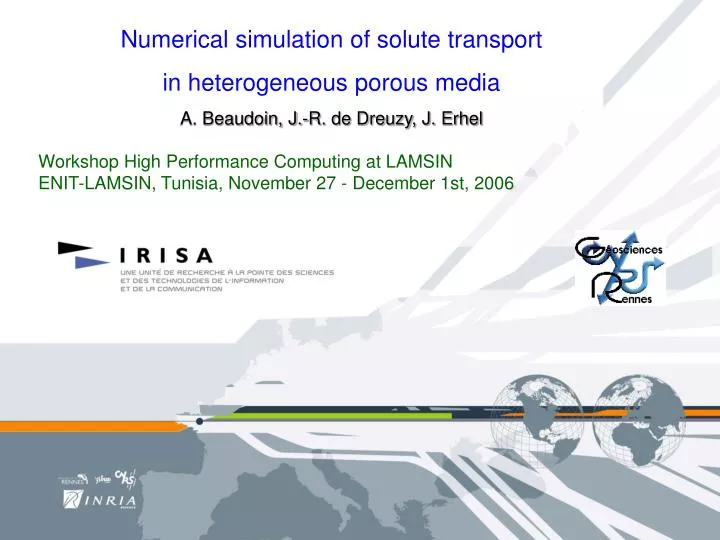
Numerical simulation of solute transport in heterogeneous porous media A. Beaudoin, J.-R. de Dreuzy, J. Erhel Workshop High Performance Computing at LAMSIN ENIT-LAMSIN, Tunisia, November 27 - December 1st, 2006
Physical model 2D Heterogeneous permeability field Stochastic model Y = ln(K) with correlation function
Nul flux Fixed head Fixed head Nul flux Flow model Steady-state case Darcy equation Mass conservation equation Boundary conditions v = - K*grad (h) div (v) = 0
Nul flux and C=0 Fixed head and dC/dn=0 Fixed head and C=0 Nul flux and C=0 Transport model Advection-dispersion equation Boundary conditions Initial condition injection dC/dt + div(v C - d gradC) = f
Numerical flow simultions Finite Volume Method with a regular mesh ; N =Nx Ny cells Large sparse structured matrix A of order N with 5 entries per row Linear system Ax=b
Numerical transport simulation Particle tracker injection Many independent particles Bilinear interpolation for v
Examples of simulations with σ=2 Pe=10 Pe=∞
Sparse direct solver memory size and CPU time with PSPASES Theory : NZ(L) = O(N logN) Theory : Time = O(N1.5) variance = 1, number of processors = 2
Multigrid sparse solver CPU time with HYPRE/AMG variance = 1, number of processors = 4 residual=10-8 Linear complexity of BoomerAMG
Transport with particle tracker CPU time variance = 1, number of processors = 4 Linear complexity of particle tracker
Sparse linear solvers Impact of permeability variance matrix order N = 106 matrix order N = 16 106 PSPASES and BoomerAMG independent of variance BoomerAMG faster than PSPASES with 4 processors
Particle tracker Impact of permeability variance and correlation length number of particles injected = 1000, Peclet number = number of processors P = 64 and matrix order N = 134.22 106 Transport CPU time increases with variance Transport CPU time slightly sensitive to correlation length
Particle tracker Impact of Peclet number and correlation length number of particles injected = 2000, variance = 9.0, number of processors P = 64 and matrix order N = 134.22 106 Transport CPU time increases for small Peclet numbers Transport CPU time slightly sensitive to correlation length
Parallel architecture Parallel architecture distributed memory 2 nodes of 32 bi – processors (Proc AMD Opteron 2Ghz with 2Go of RAM)
Parallel algorithms and Data distribution Domain decomposition into slices Ghost cells at the boundaries
Parallel algorithms and Data distribution Parallel matrix generation using FFTW Parallel sparse solver Parallel particle tracker
Direct and multigrid solvers Parallel CPU time matrix order N = 106 matrix order N = 4 106 variance = 9
Direct and multigrid solvers Speed-up matrix order N = 106 matrix order N = 4 106
Particle tracker Parallel CPU time
Flow and transport computations Summary • PSPASES is efficient for small matrices • HYPRE-AMG and PSPASES are not sensitive to the variance • HYPRE-AMG is efficient for large matrices • HYPRE-AMG and PSPASES are scalable • Particle tracker is sensitive to Peclet number • Particle tracker is efficient • transport requires less CPU time than flow for large matrices