Waves in heterogeneous media: numerical implications

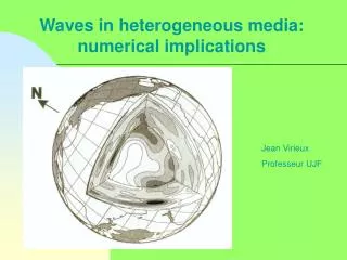
1. Waves in heterogeneous media: numerical implications Jean Virieux Professeur UJF

2. Acknowledgments • Victor Cruz-Atienza (Géosciences Azur on leave for SDSU) FDTD • Matthieu Delost (Géosciences Azur on leave) Wavelet tomography • Céline Gélis (Géosciences Azur now at Amadeous) Full wave elastic imaging • Bernhard Hustedt (Géosciences Azur now at Shell) Wavelet decomposition of PDE • Stéphane Operto (Géosciences Azur/ CNRS CR) full researcher • Céline Ravaut (Géosciences Azur now at Dublin) Full acoustic inversion • Spice group in Europe : http://www.spice-rtn.org • FDTD introduction : • ftp://ftp.seismology.sk/pub/papers/FDM-Intro-SPICE.pdf • By P. Moczo, J. Kristek and L. Halada

3. SEISMIC WAVE MODELING FOR SEISMIC IMAGING • (Very) large-scale problems. Example of hydrocarbon exploration • Target (oil & gas exploration): 20 km x 20 km x 8 km • Maximum frequency: 20 Hz • Minimum P and S wave velocities: 1.5 km/s and 0.7 km/s • FD discretization in the acoustic approximation: • h=1500/20/4 ~18 m. Dimensions of the FD grid: 1110 x 1110 x 445 • Number of degrees of freedom: 550.106 (for the scalar pressure wavefield P) • FD discretization in the elastic approximation: • h=700/20/4~9 m. Dimensions of the FD grid: 2220 x 2220 x 890 • Number of degrees of freedom: 3x4.4.109=~2x12=13.109 (for the vectorial velocity wavefield Vx, Vy, Vz) • If the wave equation is solved in the frequency domain (implicit scheme), sparse linear system should be solved, the dimension of which is the number of unknowns. Need of efficient parallel algorithms on large-scale distributed-memory platforms. Both time and memory management are key issues.

4. SEISMIC WAVE MODELING FOR SEISMIC IMAGING • (Very) large-scale problems. Example of the global earth • Target (the earth: sphere of 6370-km radius • Maximum frequency: 0.2 Hz • Hexahedric meshing: • Number of degrees of freedom: 14.6 109 (for the vectorial velocity wavefield Vx, Vy, Vz) • Simulation length: 60 minutes (50000 time steps with a time interval of 72 ms) • Simulation on 1944 processors of the Eart Simulator (Japan): • 2.5 Terabytes of memory. • MPI (Message Passing Intyterface) parallelism. • Performance: 5 Teraflops. • Wall-clock time for one simulation: 15 hours. From D. Komatitsch, J. Ritsema and J. Tromp, The spectral-element method, Beowulf computing, and global seismology, Science, 298, 2002, p. 1737-1742.

5. SEISMIC WAVE MODELING FOR SEISMIC IMAGING q Modeling in heterogeneous media: Need of sophisticated numerical schemes on unstructured meshes (finite-element-based method). Example of a shallow-water target with soft sediments on the near surface. Triangular meshing for Discontinuous Galerkin method From Brossier et al. (2009)

6. SEISMIC WAVE MODELING FOR SEISMIC IMAGING q Multi-r.h.s simulations in the context of large 3D surveys and non linear iterative optimization. Building a model by full-waveform inversion requires at least to solve three times per inversion iteration the forward problem (seismic wave modeling) for each source of the acquisition survey. Number of simulations for a realistic full-waveform inversion case study Let’s consider a coarse wide-aperture/wide-azimuth survey with a network of land stations. DR=400 m. Number of sensors (processed as sources in virtue of reciprocity of Green functions: 50x50=2500 r.h.s. The forward problem must be solved 2500 x 3=7500 per inversion iterations. Few hundreds to few thounsands of inversion iterations may be required to converge towards final models.

7. ODE versus PDE formulations Non-linear Linear O.D.E Ordinary differential Equations P.D.E Partial Differential Equations GOAL : find ways to transform differential operators into algebraic operators in order to use linear algebra at the end Symmetry between space and time ?

8. An apparent easy way Spectral methods allow to go directly to this algebraic structure Dispersion relation has to be verified BUT conditions have to be expressed in this dual space : here is the difficulty ! Pseudo-spectral approach : a remedy for a precise and fast strategy Go to the dual space only for computing spatial derivatives and goes back to the standard space for equations and conditions Frequency approach of Pratt : the opposite way around

9. One-dimensional scalar wave The scalar wave equation is verified by the vibration u(t,x) Homogeneous medium The wave solution is u(x,t)=F(x+ct)+G(x-ct) whatever are F and G (to be checked) The wave is defined by pulsation w, wavelength l, wavenumber k and frequency f and period T. We have the following relations with the dispersion relation A plane wave is defined by The phase velocity is for any frequency If the pulsationw depends on k, we have and the group velocity is which is identical to phase velocity for non-dispersive waves

10. First-order hyperbolic equation stress Let us define other variables for reducing the derivative order in both time and space The 2nd order PDE became a 1st order PDE velocity This is true for any order differential equations: by introducing additionnal variables, one can reduce the level of differentiation. Among these different systems, one has a physical meaning which becomes with Other choices are possible as displacement-stres instead of velocity-stress.

11. Characteristic variables Consider an linear system is defined by If the matrix A could be diagonalizable with real eigenvalues, the system is hyperbolic.If eigenvalues are positive, the system is strictly hyperbolic. The system could be solved for each component fp The curve x0+lp t is the p-characteristic The scalar wave introduces w=(v,s) and the following matrix w(u,d) where u design the upper solution and d the downgoing solution. The transformation from w to f splits left and right propagating waves

12. Other PDE in physics The scalar wave equation is a partial differential equation which belongs to second-order hyperbolic system. Wave Equation Fluid Equation Diffusion Equation Laplace Equation Fractional derivative Equation Time is involved in all physical processes except for the Laplace equation related to Newton law and mass distribution. Poisson equation could be considered as well when mass is distributed inside the investigated volume Poisson Equation

13. Initial and boundary conditions Initial conditions u(x,0) 1D string medium Boundary conditions u(0,t) Boundary conditions u(L,t) Dirichlet conditions on u Neumann conditions on s f(x,t) Excitation condition Difficult to see how to discretize the velocity ! Much better for handling heterogeneity

14. Finite-difference discretization grid interval: h; time interval: t Basis functions: Dirac comb

15. Physical justification of the FD method Huygen’s principle Each point of the FD grid acts as a secondary source. The envelope of the elementary diffractions provides the seismic response of the continuous medium if this latter is sufficiently-finelly discretized.

16. Exploding-reflector modeling

17. i-1 i i+1 Finite Difference Stencil Truncations errors : (Leveque 1992) Higher-order terms : same procedure but you need more and more points Second derivative

18. Discretisation and Taylor expansion Assuming an uniform discretisationDx,Dt on the string, we consider interpolation upto power 4 by summing, we cancel out odd terms neglecting power 4 terms of the discretisation steps. We are left with quadratic interpolations, although cubic terms cancel out for precision.

19. Second-order accurate central FD approximation and staggered grids EM (Yee, 1966); Earthquake (Madariaga, 1976), Wave (Virieux, 1986)

20. Higher-order accurate centred FD scheme: the 4th-order example

21. Second-order accurate Central-difference approximation Leapfrog Second-order accurate Central-difference approximation

22. Leapfrog 2nd-order accurate central-difference approximation Leapfrog 4th-order accurate central-difference approximation

23. Central-difference approximation of second partial derivative

24. Other expansions ei(x) could be any basis describing our solution model and for which we can compute easily and accurately either analytical or numerical compute derivatives A polynomial expansion is possible and coefficients of the polynome could be estimated from discrete values of u: linear interpolation, spline interpolation, sine functions, chebyshev polynomes etc Choice between efficiency and accuracy (depends on the problem and boundary conditions essentially)

25. Consistency Local error Taylor expansion around (ih,mDt) FD scheme is consistent with the differential equations (do the same for the other equation)

26. Stability analysis A numerical scheme is stable if it provides a bounded solution for a bounded source excitation. A numerical scheme is unstable if it provides an unbounded solution for a bounded source excitation. A numerical scheme is conditionnally stable if it is stable provided that the time step verifies a particular condition.

27. Stability Harmonic analysis in space and in time w is complex : the solution grows exponentially with time : UNSTABLE Local stability # long-term stability (finite domain validity) CONSISTENCE + STABILITY = CONVERGENCE (not always to the physical solution)

28. m+1 m m-1 i-1 i i+1 STABLE STENCIL :leap-frog integration Harmonic analysis is real The solution does not grow with time : STABLE CFL condition Courant, Friedrichs & Levy Magic step Dt=h/c0 Characteristic line The time step cannot be larger than the time necessary for propagating over h Von Neuman stability study

29. Long-term stability Local stability # long-term stability (finite domain validity) Long-term stability is difficult to analyze and comes from glass modes or numerical noise associated with finite discretisation Which could amplified constructively these coherent noises. Finally CONSISTENCE + STABILITY = CONVERGENCE (not always to the physical solution)

30. Time integration (more theory) Euler Backward Euler Left-side (upwind) Right-side Lax-Friedrichs Leapfrog Lax-Wendroff Beam-Warming

31. The staggered grid m+1 m m-1 i-1 i i+1 RED-BLACK PATTERN ONLY BOUNDARY CONDITIONS WOULD HAVE COUPLED THEM UNCOUPLED SUBGRID : SAVE MEMORY STAGGERED GRID SCHEME INDICE FORTRAN ? Second-order in time & in space

32. NUMERICAL DISPERSION Moczo et al (2004) How small should be h compared to the wavelength to be propagated ? 4ème ordre 2ème ordre

33. PARSIMONIOUS RULE How to define these discrete values for an heterogeneous medium ? (especially when considering strong discontinuities) How to estimate the spatial operator Do same thing for r

34. m+1 m+1 m m m-1 m-1 0 0 1 1 2 2 FREE SURFACE (Neumann condition) Amplitude deficit of wave nearby the free surface We can see that we have amplified by a factor of 2 Antisymmetric stress

35. m+1 m m-1 0 1 2 ESIM procedure Predict by extrapolation values outside the domain for keeping the finite difference stencil while verifying solutions on the boundary SAT procedure Modify the stencil when hitting the boundary for keeping same accuracy while using only values on one-side of the boundary SAT has a mathematical background while ESIM has not

36. Source or grid excitation Impulsive source The source is a term which should be added to the equation. Because it is related to acceleration, we denote it as an impulsive excitation. Known solution A particular solution of the wave equation is injected into the medium or the grid. Typically an incident plane wave is applied at each grid point along a given line. Explosive source A very popular excitation is the explosive source, which requires either applications of opposite sign forces on two nodes or a fictious force between two nodes. Once integration has been performed, we should add

37. Radiative boundaries One may assign boundary conditions as if the medium was infinite, also known as radiative conditions. These conditions may be very complex to design if the medium is heterogeneous. For the 1D case, we may simply say that which again is exactly verified for the magic step of characteristics.For other time steps, interpolation betweent-Dt and t-2Dt. In 2D and 3D, the shape of the wavefront must be introduced in an attempt for absorbing waves along boundaries and we shall see that other techniques rather radiative conditions may be considered (p-characteristics). The Perfectly Matched Layer concept turns out to be very efficient (Berenger, 1994).

38. ABC : PML conditions On conserve des variables à intégrer qui suivent la propagation dans une direction

39. Energy balance PML absorption is better than absorption by other methods at any angle of incidence (at the expense of a cost in time domain)

41. 3D test of PML conditions Left : finite box with Neuman conditions Middle : PML Right : difference between true solution and PML solution

42. STAGGERED GRID : A FATALITY 1D : Yes (for the moment!) 2D & 3D : No (one may use the spatial extension!) X Trick Z 3D case PSG FSG Combine ?

43. Saenger stencil New staggered grid sxx,szz sxz vz vx Local coupling between x and z directions: new staggered grid and velocity components define at a single node (as for the stress). Expected better behaviour for the interaction with the free surface (it has been verified).

44. FSG versus PSG PSG should be preferred when one needs all components at a single node (anisotropy, plasto-elastic formulation …)

45. NUMERICAL ANISOTROPY FSG PSG COMBINE ?

46. All you need is there • We have all ingredients for resolving partial differential equations in the FDTD domain. • Loop over time k = 1,n_max t=(k-1)*dt • Loop over stress field i=1,i_max x=(i-1)*dx • compute stress field from velocity field: apply stress boundary conditions; end • Loop over velocity field i=1,i_max x=(i-1)*dx • compute velocity field from stress field: apply velocity boundary conditions; end • Set external sources effects • compute by replacing OR by adding external values at specific points. If we replace, the input should be a solution of the wave equation. • End loop over time • Exercice : write the same organigram in the frequency domain. • Exercice : write a fortran program to solve the 1D equation (should be done in a WE).

47. COLLOCATION • FD method : discrete equations exact at nodes (strong formulations) • FE method : equations verified on the average over an element (to be defined with respect to nodes) (weak formulation) • FV method : equations verified on the average over an volume (only flux between volumes)

48. COLLOCATION FD dirac cumb FE method : elements share nodes ! FV method : elements share edges ! FV method requires simpler meshing as well as simpler message communications …. Usually this is the standard extension of FD modeling in mechanics

49. Finite volume method Pseudo-flux conservative form

50. Finite volume method