Download

1 / 29
310 likes | 540 Views
Chi-square test or c 2 test. What if we are interested in seeing if my “ crazy ” dice are considered “fair”? What can I do?. Chi-square test. Used to test the counts of categorical data Three types Goodness of fit (univariate) Independence (bivariate)

E N D
What if we are interested in seeing if my “crazy” dice are considered “fair”? What can I do?
Chi-square test • Used to test the counts of categorical data • Three types • Goodness of fit (univariate) • Independence (bivariate) • Homogeneity (univariate with two samples)
c2 distribution – df=3 df=5 df=10
c2 distribution • Different df have different curves • Skewed right • As df increases, curve shifts toward right & becomes more like a normal curve
c2 assumptions • SRS – reasonably random sample • Have countsof categorical data & we expect each category to happen at least once • Sample size – to insure that the sample size is large enough we should expect at least five in each category. ***Be sure to list expected counts!! Combine these together: All expected counts are at least 5.
c2 Goodness of fit test Based on df – df = number of categories - 1 • Uses univariate data • Want to see how well the observedcounts “fit” what we expect the counts to be • Use c2cdf function on the calculator to find p-values
Hypotheses – written in words H0: the observed counts equal the expected counts Ha: the observed counts are not equal to the expected counts Be sure to write in context!
Does your zodiac sign determine how successful you will be? Fortune magazine collected the zodiac signs of 256 heads of the largest 400 companies. Is there sufficient evidence to claim that successful people are more likely to be born under some signs than others? Aries 23 Libra 18 Leo 20 Taurus 20 Scorpio 21 Virgo 19 Gemini 18 Sagittarius 19 Aquarius 24 Cancer 23 Capricorn 22 Pisces 29 How many would you expect in each sign if there were no difference between them? How many degrees of freedom? I would expect CEOs to be equally born under all signs. So 256/12 = 21.333333 Since there are 12 signs – df = 12 – 1 = 11
Assumptions: • Have a random sample of CEO’s • All expected counts are greater than 5. (I expect 21.33 CEO’s to be born in each sign.) • H0: The number of CEO’s born under each sign is the same. • Ha: The number of CEO’s born under each sign is different. • P-value = c2cdf(5.094, 10^99, 11) = .9265 a = .05 • Since p-value > a, I fail to reject H0. There is not sufficient evidence to suggest that the CEOs are born under some signs than others.
A company says its premium mixture of nuts contains 10% Brazil nuts, 20% cashews, 20% almonds, 10% hazelnuts and 40% peanuts. You buy a large can and separate the nuts. Upon weighing them, you find there are 112 g Brazil nuts, 183 g of cashews, 207 g of almonds, 71 g or hazelnuts, and 446 g of peanuts. You wonder whether your mix is significantly different from what the company advertises? Why is the chi-square goodness-of-fit test NOT appropriate here? What might you do instead of weighing the nuts in order to use chi-square? Because we do NOT have counts of the type of nuts. We could count the number of each type of nut and then perform a c2 test.
Offspring of certain fruit flies may have yellow or ebony bodies and normal wings or short wings. Genetic theory predicts that these traits will appear in the ratio 9:3:3:1 (yellow & normal, yellow & short, ebony & normal, ebony & short) A researcher checks 100 such flies and finds the distribution of traits to be 59, 20, 11, and 10, respectively. What are the expected counts? df? Are the results consistent with the theoretical distribution predicted by the genetic model? (see next page) Since there are 4 categories, df = 4 – 1 = 3 Expected counts: Y & N = 56.25 Y & S = 18.75 E & N = 18.75 E & S = 6.25 We expect 9/16 of the 100 flies to have yellow and normal wings. (Y & N)
Assumptions: • Have a random sample of fruit flies • All expected counts are greater than 5. • Expected counts: • Y & N = 56.25, Y & S = 18.75, E & N = 18.75, E & S = 6.25 • H0: The distribution of fruit flies is the same as the theoretical model. • Ha: The distribution of fruit flies is not the same as the theoretical model. • P-value = c2cdf(5.671, 10^99, 3) = .129 a = .05 • Since p-value > a, I fail to reject H0. There is not sufficient evidence to suggest that the distribution of fruit flies is not the same as the theoretical model.
c2 test for independence • Used with categorical, bivariate data from ONEsample • Used to see if the two categorical variables are associated (dependent) or not associated (independent)
Hypotheses – written in words H0: two variables are independent Ha: two variables are dependent Be sure to write in context!
A beef distributor wishes to determine whether there is a relationship between geographic region and cut of meat preferred. If there is no relationship, we will say that beef preference is independent of geographic region. Suppose that, in a random sample of 500 customers, 300 are from the North and 200 from the South. Also, 150 prefer cut A, 275 prefer cut B, and 75 prefer cut C.
If beef preference is independent of geographic region, how would we expect this table to be filled in? 90 60 165 110 45 30
Assuming H0 is true, Expected Counts
Degrees of freedom Or cover up one row & one column & count the number of cells remaining!
Now suppose that in the actual sample of 500 consumers the observed numbers were as follows: (on your paper) Is there sufficient evidence to suggest that geographic regions and beef preference are not independent? (Is there a difference between the expected and observed counts?)
Assumptions: • Have a random sample of people • All expected counts are greater than 5. • H0: geographic region and beef preference are independentHa: geographic region and beef preference are dependent • P-value = .0226 df = 2 a = .05 • Since p-value < a, I reject H0. There is sufficient evidence to suggest that geographic region and beef preference are dependent. Expected Counts: N S A 90 60 B 165 110 C 45 30
c2 test for homogeneity • Used with a single categorical variable from two (or more) independent samples • Used to see if the two populations are the same (homogeneous)
Assumptions & formula remain the same! Expected counts & df are found the same way as test for independence. Only change is the hypotheses!
Hypotheses – written in words H0: the two (or more) distributions are the same Ha: the distributions are different Be sure to write in context!
The following data is on drinking behavior for independently chosen random samples of male and female students. Does there appear to be a gender difference with respect to drinking behavior? (Note: low = 1-7 drinks/wk, moderate = 8-24 drinks/wk, high = 25 or more drinks/wk)
Expected Counts: M F 0 158.6 167.4 L 554.0 585.0 M 230.1 243.0 H 38.4 40.6 • Assumptions: • Have 2 random sample of students • All expected counts are greater than 5. • H0: drinking behavior is the same for female & male studentsHa: drinking behavior is not the same for female & male students • P-value = .000 df = 3 a = .05 • Since p-value < a, I reject H0. There is sufficient evidence to suggest that drinking behavior is not the same for female & male students.