Maximum likelihood estimators
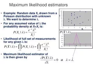
Maximum likelihood estimators. Example: Random data X i drawn from a Poisson distribution with unknown We want to determine For any assumed value of the probability density at X=X i is: Likelihood of full set of measurements for any given is:

Maximum likelihood estimators
E N D
Presentation Transcript
Maximum likelihood estimators • Example: Random data Xi drawn from a Poisson distribution with unknown We want to determine • For any assumed value of the probability density at X=Xi is: • Likelihood of full set of measurements for any given is: • Maximum likelihood estimator of isthen given by i Xi
i Xi Xi Maximum likelihood estimate of • Take logs and maximize likelihood: • Note that result is unbiased since
Variance of ML estimate • Algebra of random variables gives • This is a minimum-variance estimate -- it’s independent of and • Important note: the error bars on the Xi are derived from the model, not from the data!
Xi i Error bars attach to the model, not to the data! • Example: Poisson data Xi . • How can you attach an error bar to the data points? • The right way: • is the mean count rate predicted by the model. • The wrong way: if you assign • then when Xi=0, (0)=0, giving: • Assigning (Xi )= √Xi gives a downward bias because points lower than average get smaller error bars, and hence more weight than they deserve.
Confidence interval on a single parameter • The 1 confidence interval on includes 68% of the area under the likelihood function: L() 2 2
Fitting a line to data – 1 • Fit a line y = ax + b to a single data point: • Blue lines have 2 = 0 • Red lines have 2 = 1 • 2 contours in the (a,b) plane look like this: • Solution is not unique, since 2 parameters are constrained by only 1 data point. • Bayes: prior P(a,b) will determine value of a. b 2 = 1 2 = 0 2 = 1 a
b y 2 = 2 2 = 0 b a x Fitting a line to data – 2a • Fitting a line y = ax + b to 2 data points: • red lines give 2 = 2 • blue line gives 2 = 0 • Note that a, b are not independent. All solutions (a,b) lying on red ellipse give 2 = 2
Independent vs. correlated parameters • a and b are not independent in this example. • To find the optimal (a,b) we must: • minimize 2 with respect to a at a sequence of fixed b • then minimise the resulting 2 values with respect to b. • If a and b were independent, then all slices through the 2 surface at each fixed b would have same shape. • Similarly for a. • So we could optimize them independently, saving a lot of calculation. • How can we make a and b independent of each other?
y b 2 = 2 2 = 0 b a x Fitting a line to data – 2b • Fitting a line y = a(x-x) + b to 2 data points: • red lines give 2 = 2 • blue line gives 2 = 0 • Note that a, b are now independent. All solutions (a,b) lying on red ellipse give 2 = 2
Intercept and slope for independent a, b • Intercept: • Slope: 2 2 a b b a
Choosing orthogonal parameters • Good practice. • Results for any one parameter don’t depend on values of other parameters. • Example: fitting a gaussian profile. Parameters to be fitted are: • Width, w • Area or peak value. Which is best? Peak value depends on width – bad P A Area is independent of width – good