Maximum Likelihood Estimation in Statistics: Understanding Parameters
Learn about Maximum Likelihood Estimation (MLE) in statistics, how it helps estimate parameters from sample data, including Bernoulli, Multinomial, and Gaussian distributions. Explore methods to evaluate estimators for bias and variance.


Maximum Likelihood Estimation in Statistics: Understanding Parameters
E N D
Presentation Transcript
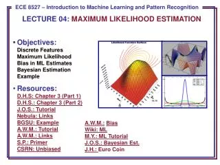
Maximum Likelihood Estimation Berlin Chen Department of Computer Science & Information Engineering National Taiwan Normal University References: 1. Ethem Alpaydin, Introduction to Machine Learning , Chapter 4, MIT Press, 2004
Population (sample space) Sample Inference Statistics Parameters Sample Statistics and Population Parameters • A Schematic Depiction
Introduction • Statistic • Any value (or function) that is calculated from a given sample • Statistical inference: make a decision using the information provided by a sample (or a set of examples/instances) • Parametric methods • Assume that examples are drawn from some distribution that obeys a known model • Advantage: the model is well defined up to a small number of parameters • E.g., mean and variance are sufficient statistics for the Gaussian distribution • Model parameters are typically estimated by either maximum likelihood estimation (MLE) or Bayesian (MAP) estimation
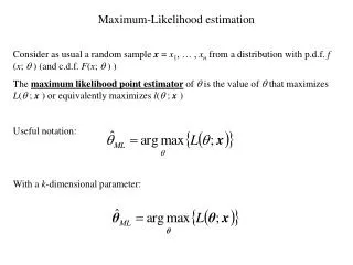
Maximum Likelihood Estimation (MLE) (1/2) • Assume the instances are independent and identically distributed (iid), and drawn from some known probability distribution • : model parameters (assumed to be fixed but unknown here) • MLE attempts to find that make the most likely to be drawn • Namely, maximize the likelihood of the instances
MLE (2/2) • Because logarithm will not change the value of when it take its maximum (monotonically increasing/decreasing) • Finding that maximizes the likelihood of the instances is equivalent to finding that maximizes the log likelihood of the sample instances( that best fits the instances) • As we shall see, logarithmic operation can further simplify the computation when estimating the parameters of those distributions that have exponents
Bernoulli Distribution A random variable takes either the value (with probability ) or the value (with probability ) Can be thought of as is generated form two distinct states The associated probability distribution The log likelihood for a set of iid instances drawn from Bernoulli distribution MLE: Bernoulli Distribution (1/3)
MLE: Bernoulli Distribution (2/3) • MLE of the distribution parameter • The estimate for is the ratio of the number of occurrences of the event ( ) to the number of experiments • The expected value for • The variance value for
MLE: Bernoulli Distribution (3/3) • Appendix A The maximum likelihood estimate of the mean is the sample average
MLE: Multinomial Distribution (1/4) • Multinomial Distribution • A generalization of Bernoulli distribution • The value of a random variable can be one of K mutually exclusive and exhaustive states with probabilities , respectively • The associated probability distribution • The log likelihood for a set of iid instances drawn from a multinomial distribution
MLE: Multinomial Distribution (2/4) • MLE of the distribution parameter • The estimate for is the ratio of the number of experiments with outcome of state ( ) to the number of experiments Urn
MLE: Multinomial Distribution (3/4) • Appendix B Lagrange Multiplier =1 Lagrange Multiplier: http://www.slimy.com/~steuard/teaching/tutorials/Lagrange.html
MLE: Multinomial Distribution (4/4) Urn P(B)=3/10 P(W)=4/10 P(R)=3/10
MLE: Gaussian Distribution (1/3) • Also called Normal Distribution • Characterized with mean and variance • Recall that mean and variance are sufficient statistics for Gaussian • The log likelihood for a set of iid instances drawn from Gaussian distribution
MLE: Gaussian Distribution (2/3) • MLE of the distribution parameters and • Remind that and are still fixed but unknown sample average sample variance
MLE: Gaussian Distribution (3/3) • Appendix C
Evaluating an Estimator : Bias and Variance (1/6) • The mean square error of the estimator can be further decomposed into two parts respectively composed of bias and variance constant constant 0 variance bias2
Evaluating an Estimator : Bias and Variance (3/6) • Example 1: sample average and sample variance • Assume samples are independent and identically distributed (iid), and drawn from some known probability distribution with mean and variance • Mean • Variance • Sample average (mean) for the observed samples • Sample variance for the observed samples for discrete random variables estimator estimate ?
Evaluating an Estimator : Bias and Variance (4/6) • Example 1 (count.) • Sample average is an unbiased estimator of the mean • is also a consistent estimator:
Evaluating an Estimator : Bias and Variance (5/6) • Example 1 (count.) • Sample variance is an asymptotically unbiased estimator of the variance
Evaluating an Estimator : Bias and Variance (6/6) • Example 1 (count.) • Sample variance is an asymptotically unbiased estimator of the variance The size of the observed sample set
Bias and Variance: Example 2 different samples for an unknown population error of measurement
Big Data => Deep Learning (Deep Neural Networks, etc.) complicated or sophisticated modeling structures Simple is Elegant ? Occam’s razor favors simple solutions over complex ones.