Download
1 / 23
230 likes | 317 Views
Explore the implementation of an MPEG1 Layer III (MP3) decoder on x86 and TMS320C6711 platforms, decoding steps, frame structure, Huffman decoding, requantization, and stereo processing.

E N D
Developement and Implementation of an MPEG1 Layer III Decoder on x86 and TMS320C6711 platforms BraidottiEnrico (Farina Simone)
What is MPEG1 Layer III ? • Frequently referred to as “MP3” • Method to store compressed audio (LOSSY ) • Developed by Moving Pictures Expert Group (MPEG) • Standard ISO/IEC 11172-3 (Audio Part 3), 1991 • Compression rate w/out recognizeable quality loss up to 12x • Last release of MPEG1 family: • Highest complexity • Provides best quality
Standard MPEG1 • 3 possible compression types (increasing complexity): • Layer I • Layer II • Layer III • Sampling frequencies for Layer III: • 32 kHz • 44.1 kHz • 48 kHz • Bitrates: • Min 32 kbit/s • Max 320 kbit/s Compact Disc: 1.41 Mbit/s
BITSTREAM FORMAT • Whole bitstream is divided into frames of defined length: • framesize = 144· bitrate / sampling frequency + padding (bytes) • Frames are divided in 2 granules and are composed by different parts: • Header • CRC (optional) • Side Information • Main data • Ancillary data (optional)
FRAME HEADER • Syncword =12 bits put to ‘1’ • ID =1 for MPEG1 Audio (2 bits used for MPEG2 and 2.5) • Padding = to adjust framesize (and effective bitrate • of CBR files)
SIDE INFORMATION • Length depends on number of channels • 17 bytes for single channel • 32 bytes for others • Contains all necessary informations for decoding the • Main data section • Main structure is:
BIT RESERVOIR It is one of the most important features of Layer III format and it works as follows (use of main_data_end ):
MAIN DATA • SCALEFACTORS • informations in the Side Information section • HUFFMAN CODED DATA • extraction of scaled frequency lines (not ordered in some cases)
DECODING STEPS • SYNCHRONIZATION • HEADER DECODING • SKIPPING CRC (if present) • SIDE INFO DECODING • SCALEFACTORS DECODING
HUFFMAN DECODING • Lossless-type coding / decoding • Fixed – variable • Based on 18 Huffman Tables (specific for MPEG1) • Codewords up to 19-bit long • Tables up to 256 values
HUFFMAN DECODING • Big Values • Region 0 • Region 1 • Region 2 • Count 1 • RZero
HUFFMAN DECODING Couple of f. lines ( big-values ) Quadruple of f. lines ( count1 )
HUFFMAN DECODING • CLUSTERED HUFFMAN DECODING (R. Hashemian ) • Compromise between binary-tree and direct look-up • decoding • Custom made Huffman tables containing 16-bit words • Structure of words depend on HIT / MISS:
HUFFMAN DECODING Example Clustered Table 1 Huffman Table 1 xylencodeword 0 0 1 1 0 1 3 001 1 0 2 01 1 1 3 000
REQUANTIZATION (DESCALING) The Huffman decoded frequency lines are restored to their original values according to the following formulas:
REQUANTIZATION (DESCALING) • Use of large look-up table with all possible values of modulus of Huffman decoded data (0 → 15 + 213 = 8206) • pros: speed, accuracy • cons: memory requirements (32 KByte with float precision) Reduced Look-up table • pros: table is 87.5 % smaller (4 KByte with float precision) • cons: speed (need to calculate is· 0.125), accuracy
REQUANTIZATION (DESCALING) • Shift – based power computing (T. Uželac ) • Requantization has to be done up to 2304 times each frame, direct computation of: would require too many clock cycles
REQUANTIZATION (DESCALING) • shift operations • 2 small look-up tables (total of 32 Bytes) scale = scalefac_scale + 1; a = global_gain - 210 - (scalefac_long << scale); if (preflag) a -= (pretab << scale); if (a < -127) y = 0; if (a >= 0) y = tab[a&3]*(1 << (a >> 2)); else y = tabi[(-a)&3]/(1 << ((-a) >> 2)); tab contains values: [20, 21/4, 21/2, 23/4] tabi contains values: [20, 2-1/4, 2-1/2, 2-3/4]
STEREO PROCESSING • INTENSITY STEREO • In the critical bands higher than 2 kHz, the sensation of stereo is given mainly by the envelope of the signal. • The encoder codes only one sum - like signal and the decoder extracts separate L and R with different scalefactors • MIDDLE/SIDE STEREO • Encoding of the Middle (L+R) and Side (L-R) signals for reducing redundant elements
STEREO PROCESSING • There are 4 different typologies of transmission for stereophonic signals (according to mode_extension, found in the header ):
STEREO PROCESSING • MIDDLE/SIDE STEREO • Left and Right channels are simply reconstructed according to: • INTENSITY STEREO • Values are read from the Rzero part of Left channel and IS positions is_pos (sfb ) are read from scalefactors of right channel:
REORDERING It is performed only when using short blocks: this is due to the way the MDCT in the encoder arranges the output lines.