Decoder Implementation
Cell 1 Cell 2. t i+1. t i. 0,7. 7,7. 13. (5,4). 41. 0,0. 7,0. Decoder Implementation. Transition during any one time interval can be grouped into disjoint cells Branch Metrics aa’ ab’ ca’ cb’ bc’ bd’ dc’ dd’ Hamming distance for HD

Decoder Implementation
E N D
Presentation Transcript
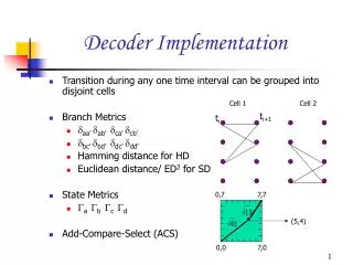
Cell 1 Cell 2 ti+1 ti 0,7 7,7 13 (5,4) 41 0,0 7,0 Decoder Implementation • Transition during any one time interval can be grouped into disjoint cells • Branch Metrics • aa’ab’ ca’ cb’ • bc’ bd’ dc’dd’ • Hamming distance for HD • Euclidean distance/ ED2 for SD • State Metrics • a b c d • Add-Compare-Select (ACS)
c a ca’ cb’ aa’ ab’ + + + + Compare Compare ˆ ˆ ˆ ˆ mc ma mc ma Select 1-of-2 Select 1-of-2 Select 1-of-2 Select 1-of-2 a’ b’ mb’ ma’ ˆ ˆ To another logic unit To another logic unit Add Compare Select (ACS)Cell 1
Free Distance • Minimum free distance minimum distance in the set of all arbitrary long paths that diverge and remerge from the all-zero path. • Systematic code free distance < Non-Systematic code free distance • Error correcting capability t = (df -1)/2
Coding Gain • Soft Decision ML decoding • Pe Q ( df/2 ) ; for moderate to high SNR • Asymptotic Coding gain G • G (dB) = 20 log10 (d f/ d ref) or G (dB) = 10 log10 (d f2/ d ref2) • Alternately for high SNR and given error probability • G (dB) = (Eb/No)U (dB) - (Eb/No)C (dB) • TCM goal to achieve d f > d ref at same info rate , BW & power
2 3 A0 1 d0= 2 sin(/8) = 0.765 4 0 1 5 2 7 B0 d1= 2 6 3 B1 1 4 d1= 2 0 5 7 6 2 C0 C1 C2 1 3 C3 4 0 5 7 d2= 2 d2= 2 6 Set Partitioning – Example of 8-PSK
States 0 0 0 C0 C1 4 4 4 2 2 2 0 4 2 6 6 6 6 C2 C3 2 2 2 6 6 6 0 0 0 4 4 4 1 5 3 7 1 1 1 C1 C0 5 5 5 2 6 0 4 3 3 3 3 3 3 7 7 7 7 7 7 1 1 1 C3 C2 5 5 5 3 7 1 5 4-State Trellis 0,1,2,3,4,5,6,7 Waveform Numbers
Coding gain for 8-PSK 4-State trellis • Candidate error event paths • 2, 1, 2 • d2 = d12 + d02 + d12 = 2 + 0.585 + 2 = 4.585 • d = sqrt( 4.585) = 2.2 • 4 • d = 2 • df min ( 2.2, 2 ) = 2, dref 2 • G (dB) = 10 log10 (d f2/ d ref2) = 3 dB
State 0426 1537 4062 5173 2604 3715 6240 7351 0 0 0 7 6 Coded 8- PSK 8 - State trellis • Coded 8-state 8-PSK • d2 = d12 + d02 + d12 = 2 + 0.585 + 2 = 4.585 df = 4.585 dref = 2 G (dB) = 10 log10 (d f2/ d ref2) = 3.6 dB 6 16-state trellis 4.1 dB coding gain over uncoded 4-PSK
Mapping Waveforms to Trellis Transitions • If k bits are to be encoded per modulation interval, trellis must allow for 2k possible transitions from each state to successor state, • More than one transition may occur between pairs of states, • All waveforms should occur with equal frequency and with a fair amount of regularity and symmetry, • Transitions originating from the same state are assigned waveforms either from subset B0 or B1 – never a mixture between them , • Transitions joining into the same state are assigned waveforms either from subset B0 or B1 – never a mixture between them , • Parallel transitions are assigned waveforms either from subset C0 or C1 or C2 or C3 – never a mixture between them.
d0 = 2 / 10 = 0.632 d1 = 2 d0 d2 = 2 d1 = 2 d0 d3 = 2 d2
State 0 4 2 6 1 5 3 7 4 0 6 2 5 1 7 3 2 6 0 4 3 7 1 5 6 2 4 0 7 3 5 1 8-state trellis for 16-QAM