Download
1 / 31
310 likes | 482 Views
Changes of Seasonal Predictability Associated with Climate Change. Kyung Jin and In-Sik Kang Climate Environment System Research Center Seoul National University. Background and Objective. International Climate of the Twentieth Century Project (C20C).

E N D
Changes of Seasonal Predictability Associated with Climate Change Kyung Jin and In-Sik Kang Climate Environment System Research Center Seoul National University
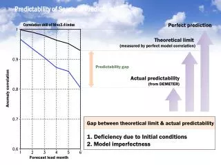
Background and Objective • International Climate of the Twentieth Century Project (C20C) • International project coordinated by Hadley Centre and COLA • Goal: Characterize climate variability and predictability of the last ~130 years through analysis of observational data and ocean-forced atmospheric general circulation models (AGCM) • “Classic” experimental design: Hadley Centre provides HadISST1.1 SST and sea ice data as lower boundary conditions - Integrate over 1871-2002 (at least 1949-2002) - Ensembles of at least 4 members • In this study, we examine • Changes of potential seasonal predictability in 100-year AGCM ensemble simulation • Plausible sources of regulation of potential predictability in AMIP run • Perfect Model Correlation • Average of correlations between each member and ensemble mean using other members in the ensemble simulations of GCM • Hence, it can be the indication of upper limit of GCM potential predictability due to SST boundary forcing • Change of Predictability following to the use of different climatology
Model Description and Experimental Design • SNU/KMA Global Climate Prediction System (GCPS) • Performed Experimental Design in SNU/GCPS • International Climate of the Twentieth Century Project (C20C) • Integration Period: Jan 1897 to Nov 1998 • Boundary Conditions • HadSST and Sea ice 1.1 (Jones et al. 2001) • PCMDI vertical ozone distribution • Atmospheric CO2 concentration: 321.07 ppm (100-yr mean) • Used Model Dataset
CES/SNU Linear Trend of Surface Temperature Oberved trend : 0.61oC/100yr Simulated trend: 0.55oC/100yr • Using anomaly data subtracted the climatology during 1961-1990 • Observation comes from CRU surface temperature and Hadley SST
Perfect Model Correlation of DJF Anomalies over Global region Global Pattern Correlation (a) Surface Temperature 1921-1950 1968-1997 0.38 0.63 • Perfect Model Correlation • Considering one member of the ensemble as an observation • Making spatial correlation between the model observation and the ensemble mean of the other members • Average of correlations between each member and ensemble mean using other members in the ensemble simulations of GCM. • Perfect Model Correlation • Average of correlations between each member and ensemble mean using other members in the ensemble simulations of GCM • Hence, it can be the indication of upper limit of GCM potential predictability due to SST boundary forcing • Change of Predictability following to the use of different climatology (b) Precipitation 0.53 0.66
Perfect Model Correlation of DJF Anomalies over Global region Global Pattern Correlation (a) Surface Temperature 1921-1950 1968-1997 0.38 0.63 • 5-year running mean • Not shown here, the increase is also detected in the case of boreal summer, even though the difference is rather weak. • The changes of predictability due to the use of different climatology is negligible in this case. • 5-year running mean (b) Precipitation 0.53 0.66
Perfect Model Correlation of AGCMs DJF PRCP Anomalies over Global region Global Pattern Correlation (a) Surface Temperature SNU NSIPP 1921-1950 1968-1997 0.38 0.44 0.63 0.65 • 5-year running mean • In NSIPP results, the ascent of potential predictability is also shown, and moreover, the interannual variability of predictability is also coincide with that of SNU. • Increase of potential predictability of recent years can be the general feature of GCM ensemble simulations. • The change of SST as the boundary condition for two models, has to be estimated to fine the origin of predictability. • In NSIPP results, the ascent of potential predictability is also shown, and moreover, the interannual variability of predictability is also coincide with that of SNU. • Increase of potential predictability of recent years can be the general feature of GCM ensemble simulations • The change of SST as the boundary condition for two models, has to be estimated to fine the origin of predictability • 5-year running mean (b) Precipitation 0.53 0.58 0.66 0.73
Forced variance Climate signals caused by external forcing Free variance Intrinsic transients due to natural variability Analysis of Variance: SNU DJF PRCP – P1(1921-1950) vs. P2(1968-1997) 1921-1950 1968-1997 (b) Forced variance (a) Forced variance (c) Free variance (d) Free variance (e) Forced/Free variance (f) Forced/Free variance • The improvement of potential predictability is coming from the increase of forced part generated by SST. The SST has an important role to regulate the potential predictability in model results.
Ratio of Temporal Perfect Model Correlation – SNU (1968-1997) vs. (1921-1950) JJA DJF (c) Surface Temperature (a) Surface Temperature (d) Precipitation (c) Precipitation • : • Red denotes that latter (1968-1997) period show higher predictability than former (1921-1950) period and blue denotes to the contrary. COR1968-1997 and COR1921-1950 means perfect model temporal correlation during 1968-1997 and 1921-1950, respectively.
Plausible Source of Improvement of Potential Predictability in AMIP run Two periods during 30 years 1921-1950 vs. 1968-1997 Improvement of Potential Predictability To find the origin of interannual characteristics of predictability Increase of Forced Variance Plausible Source • Increase of Global Mean SST Change of climatological SST field Change of SST boundary forcing • Increase of Tropical Forcing over Eastern Pacific Increase of remote forcing to whole globe • Increase of Intensity of SST variability Increase of variability of absolute value of SST anomalies
DJF Global Perfect Model Correlation and Global SST DJF Global Pattern Correlation (a) Surface Temperature • The improved predictability roughly looks some connection with global warming trend, but inconsistencies exist in the sense of interannual predictability. • 5-year running mean (b) Precipitation Perfect Model Corr. Global Mean SST
Red denotes that latter (1968-1997) period show larger variability than former (1921-1950) period and blue denotes to the contrary. Mean Absolute Value of SST Anomalies – P1(1921-1950) vs. P2(1968-1997) Mean of Absolute Value of DJF SST anomalies during 30 years (a) 1921-1950 (e) Ratio (b)/(a) (b) 1968-1997
It show the clear intensification of SST variability for latter period including both increase of intensity and frequency of ENSO and warming trend over the Indian Ocean. Longitude-Time Cross section of SST Anomalies over 5oN-5oS (b) 1968-1997 (a) 1921-1950
Regression of the Absolute Value of DJF SST Anomalies by Perfect Model Correlation (a) Global pattern correlation of rainfall • The region of SST variability regulating the potential predictability in AGCM is almost same for various variables and regions. • The interannual variability of SST over the eastern Pacific looks to have an important role for predictability. (b) PNA PRCP (c) Monsoon PRCP (d) Global 500hPa GPH (e) Monsoon 500hPa GPH
Characteristics of improved predictability - The improvement of predictability during ENSO years are clear for both El Nino and La Nina. • Even in the normal year, latter period (1968-1997, blue dots) show higher predictability than former years (1921-1950, red dots). Relationship between DJF Global PRCP Perfect Model Correlation and SST (a) Global Mean SST (b) NINO3.4 Index DJF Global Pattern Correlation of Precipitation (c) Absolute value of NINO3.4 DJF SST anomalies
PM Corr. 1 σ NINO 3.4 Composite of Absolute Value of DJF SST Anomalies by PRCP Predictability 1921-1950 1968-1997 (a) High Skill (b) High Skill (c) Ratio of (b)/(a) (d) Low Skill (e) Low Skill (f) Ratio of (e)/(d) • 8 cases are selected for high and low skill, respectively • Using 1897-1997 Climatology for both periods
Composite of Absolute Value of DJF SST Anomalies by PRCP Predictability 1921-1950 1968-1997 (a) High Skill for Normal Year (b) High Skill for Normal Year (c) Ratio of (b)/(a) (d) Low Skill for Normal Year (e) Low Skill for Normal Year (f) Ratio of (e)/(d) • 5 cases are selected for high and low skill in normal year (not ENSO), respectively • Even in the normal cases, the increase of tropical SST variability is traced. In Particular, low skill case show much larger increase over the whole tropical ocean. It is well matched with the previous results showing the higher predictability for recent years even in the non-ENSO years having small value of NINO index.
Summary • In AGCM ensemble simulations for 20th century, the increase of potential predictability is clearly shown, especially for the surface variables. • As the plausible causes of this, the change of characteristics of SST following to the global climate change can be considered: Global warming trend, intensity of ENSO activity, and the amplitude of SST anomalies are considered. • The potential predictability over the globe is very much related to the intensity of ENSO. • The magnitudes of SST anomalies over the tropics are also important for the predictability for even non-ENSO years. • To quantify the effect of each origins exactly, model experiments using regulated SST boundary condition and statistical approach are needed.
Model Experiment • Boundary Condition: 1921-1950 Climatology + 1968-1997 Anomaly • 30 years simulation with 4 ensemble member Perfect Model Corr. Global Mean SST New experiment New experiment SST
Model Experiment • Boundary Condition: 1921-1950 Climatology + 1968-1997 Anomaly • 30 years simulation with 4 ensemble member Perfect Model Corr. NINO3.4 Index New experiment New experiment SST
Perfect Model Correlation of AGCMs DJF PRCP Anomalies over Global region Global Pattern Correlation for DJF Precipitation (a) Surface Temperature SNU NSIPP 1921-1950 1968-1997 0.38 0.44 0.63 0.65 • Perfect Model Correlation • Average of correlations between each member and ensemble mean using other members in the ensemble simulations of GCM. • Hence, it can be the indication of upper limit of GCM potential predictability due to SST boundary forcing. • Change of predictability following to the use of different climatology is not detected. • Perfect Model Correlation • Average of correlations between each member and ensemble mean using other members in the ensemble simulations of GCM • Hence, it can be the indication of upper limit of GCM potential predictability due to SST boundary forcing • Change of Predictability following to the use of different climatology (b) Precipitation 0.53 0.58 0.66 0.73
Climatology of DJF SST– (1921-1950) vs. (1968-1997) DJF Climatology of SST (a) 1921-1950 (e) Difference (b) - (a) (b) 1968-1997
Perfect Model Correlation of SNUGCM DJF PRCP Anomalies SNU Pattern Correlation for DJF Precipitation (a) Surface Temperature • Global Region (0-360oE, 90oS-90oN) • Asian Monsoon Region (40-160oE, 20oS-40oN) • 5-year running mean (b) Precipitation
For the EOF analysis of analysis of variance, 1914in x-axis denotes analysis of variance during 1899-1928. EOF analysis of 30-yearr ANOVA of DJF PRCP Forced Variance Ratio of Forced/Free Variance (a) 1st mode (b) 1st mode (c) PC time series (d) PC time series
DJF Global Perfect Model Correlation and NINO3.4 Index DJF Global Pattern Correlation (a) Surface Temperature (b) Precipitation Perfect Model Corr. NINO3.4 Index
Perfect Model Correlation of SNUGCM DJF PRCP Anomalies over Global region 0.53 0.58 0.66 0.73 Using 1897-1997 Climatology
Perfect Model Correlation of SNUGCM DJF PRCP Anomalies Using 1897-1997 Climatology for both periods
Analysis of Variance – SNU DJF Z500 - P1(1921-1950) vs. P2(1968-1997)
Analysis of Variance – NSIPP DJF PRCP – P1(1930-1950) vs. P2(1968-1997)
Analysis of Variance – NSIPP DJF Z500 – P1(1930-1950) vs. P2(1968-1997)
5 cases are selected for high and low skill in normal year (not ENSO), respectively • Using 1921-1950 and 1968-1997 Climatology, respectively Composite of Absolute Value of DJF SST Anomalies by PRCP Predictability 1921-1950 1968-1997 (a) High Skill for Normal Year (b) High Skill for Normal Year (c) Ratio of (b)/(a) (d) Low Skill for Normal Year (e) Low Skill for Normal Year (f) Ratio of (e)/(d)