Seasonal Climate Predictability in Watersheds of the Upper Colorado River Basin

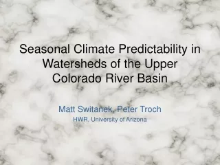
1. Seasonal Climate Predictability in Watersheds of the Upper Colorado River Basin Matt Switanek, Peter Troch HWR, University of Arizona

2. Motivation • As we all know, most (~90%) of the Colorado River water originates from the Upper Basin. • Furthermore, the Climate Prediction Center’s seasonal climate forecast skill (winter) is weak to non-existent in the Upper Basin. The CPC relies heavily on ENSO for their seasonal forecasts of precipitation and temperature. Since this relationship is typically weak in most of the Upper Basin, they observe very low to no skill in contrast to the climatology.

3. Motivation • Can we provide climate information to the CBRFC that is more skillful that what is provided now by the Climate Prediction Center? • In this effort, we decided to focus on improving skill (over the CPC) in retrospectively forecasting winter (October-March) precipitation and temperature for the Gunnison, San Juan and Green watersheds.

4. ENSO and Precipitation • Most of the Upper Colorado Basin does not see a strong relationship between ENSO and precipitation. 1901-2009 1941-1970 1971-2000 • Where does this lead?

5. CPC’s Precipitation Skill http://hydis6.hwr.arizona.edu/ForecastEvaluationTool/ Showing Ranked Probability Skill Score which assesses the skill of probabilistic forecats.

6. Establish a Longer Time Series of Precipitation and Temperature • This is because we wanted to train our model on decades worth of retrospective forecasts. Provided only 30 years of data for the testbed watersheds, we would like to use PRISM data which then would provide ~110 years. How similar are the data sets and can results obtained using PRISM be extended to the testbed data provided?

7. SST Correlations with Gunnison Winter Precipitation • Now, instead of correlating ENSO with regional precipitation, we do the reverse and correlate winter Gunnison precipitation with the preceding season’s global SSTs. • Example showing correlations between March-August SSTs with October-March Precipitation in the Gunnison (1971-2000).

8. SST Correlations with Gunnison Winter Precipitation • ENSO is not strongly correlated with winter precipitation in the Gunnison • However, we see other regions with stronger statistical relationships. Can these be used to provide skillful forecasts?

9. Using Regions of Highest Correlation 1971-2000 Time Series 2: SSTs in 2001 (March-August) that historically were most negatively correlated with winter Gunnison precipitation. SSTs expressed as standard deviations from the means at each respective location. Time Series 1: SSTs in 2001 (March-August) that historically were most positively correlated with winter Gunnison precipitation. SSTs expressed as standard deviations from the means at each respective location.

10. Building the Model 4 Parameters Positively Correlated Time Series Negatively Correlated Time Series Parameter 1: The threshold size. Values below a specified standard deviation will be thrown out. Similarly to a strong El Niño or La Niña. Parameter 2: Value which weights the overall contribution of the positively correlated time series. Parameter 3: The threshold size. Values below a specified standard deviation will be thrown out. Similarly to a strong El Niño or La Niña. Parameter 4: Value which weights the overall contribution of the negatively correlated time series.

11. Building the Model For example: Current time -> September, 2001. We want to forecast October-March precipitation. We use the most positively and negatively correlated time series from 1971-2000. To illustrate, assume we have the SSTs from the positively correlated regions expressed as standard deviations from the means at each respective location. Take the mean of the time series. Here it is -.4 Threshold = 1.5

12. Building the Model • We obtained a value of -.4 for the current time as a representation of the entire positively correlated time series. • With the same procedure, though not necessarily the same threshold, say we obtain a value of -.8 from the negatively correlated time series. Parameter 1 = 1.5 Parameter 2 = 1.7 Parameters 3 and 4 Deterministic Forecast Oct, 2001 – Mar, 2002 = .5 * -.4 +-.6 * -.8 =.28 Positive Negative Probabilistic Forecast = .28 with the standard deviation of the climatology

13. Training the Model • We used retrospective forecasts for the years 1931-1974 to establish which parameters provided the highest skills. • This was done for October-March precipitation and temperature for the Gunnison, San Juan and Green watersheds. • The more recent times were weighted a little more heavily in calculating the skills. This was another way of dealing with non-stationarity.

14. Gunnison Forecasts and Observations >50% of the time the Predictions are closer to the Observations than the climatology is to the Observations. True for all cases. This is important because the skill measures that we use more strongly reward the Predictions that are closer to extreme values than the climatology.

15. San Juan Forecasts and Observations

16. Green Forecasts and Observations

17. Winter Precipitation Skills Precipitation Salt RPSS CPC = .10 RPSS PM = .25

18. Winter Temperature Skills Temperature

19. What Now? • Implement an efficient algorithm to obtain optimum parameters. • Investigate further how non-stationarity influences each case. We then can apply the correct weights for each time step of the retrospective forecasts. For example, weighting more heavily the most positively correlated SST grid cells might not always provide higher skill. We need to be able to pick up on a transition of using more the positively correlated regions to the negative ones. The model needs to be adaptive to changing relationships. Think of how land use change at a specific time might influence a parameter that governs infiltration.

20. What Now? • If we find similar improvements in skill for each of the watersheds of the Upper Basin, can these retrospective forecasts of winter precipitation and temperature be used by the CBRFC to provide more skillful forecasts of Spring water quantity? • What about directly forecasting streamflow using this type of model? • Continue tweaking the existing methodology to see if skill can further be improved.

21. Questions / Comments / Suggestions