Download
1 / 24
301 likes | 842 Views
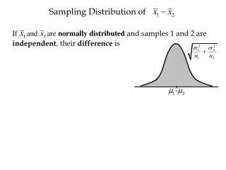
Chapter 8.6. Sampling Distribution of S 2. Sampling Distribution of S 2. If S 2 is the variance of a random sample of size n taken from a normal population having the variance σ 2 , then the statistic. has a chi-squared distribution with v = n – 1 degrees of freedom. Chapter 8.6.

E N D
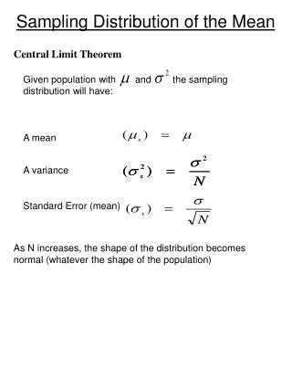
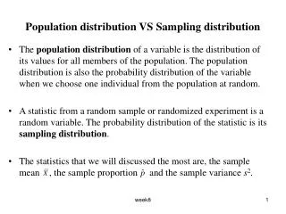
Chapter 8.6 Sampling Distribution of S2 Sampling Distribution of S2 • If S2 is the variance of a random sample of size n taken from a normal population having the variance σ2, then the statistic has a chi-squared distribution with v=n–1 degrees of freedom.
Chapter 8.6 Sampling Distribution of S2 Sampling Distribution of S2 • Table A.5 gives values of for various values of α and v. • The column headings are the areas α. • The left column shows the degrees of freedom. • The table entry are the value.
Chapter 8.6 Sampling Distribution of S2 Table A.5 Chi-Squared Distribution
Chapter 8.6 Sampling Distribution of S2 Table A.5 Chi-Squared Distribution
Chapter 8.6 Sampling Distribution of S2 Sampling Distribution of S2 A manufacturer of car batteries guarantees that his batteries will last, on the average, 3 years with a standard deviation of 1 year. If five of these batteries have lifetimes of 1.9, 2.4, 3.0, 3.5, and 4.2 years, is the manufacturer still convinced that his batteries have a standard deviation of 1 year? Assume that the battery lifetime follows a normal distribution. • From the table, 95% of the χ2 values with 4 degrees of freedom fall between 0.484 and 11.143. • The computed value with σ2=1 is reasonable. • The manufacturer has no reason to doubt the current standard deviation.
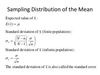
Chapter 8.7 t-Distribution t-Distribution • In the previous section we discuss the utility of the Central Limit Theorem to infer a population mean or the difference between two population means. • These utility is based on the assumption that the population standard deviation is known. • However, in many experimental scenarios, knowledge of σ is not reasonable than knowledge of the population mean μ. _ • Often, an estimate of σ must be supplied by the same sample information that produced the sample average x. • As a result, a natural statistic to consider to deal with inferences on μ is
Chapter 8.7 t-Distribution t-Distribution • If the sample size is large enough, say n≥30, the distribution of T does not differ considerably from the standard normal. • However, for n<30, the values of S2 fluctuate considerably from sample to sample and the distribution of T deviates appreciably from that of a standard normal distribution. • In the case that sample size is small, it is useful to deal with the exact distribution of T. • In developing the sampling distribution of T, we shall assume that the random sample was selected from a normal population, where
Chapter 8.7 t-Distribution t-Distribution • Let Z be a standard normal random variable and V a chi-squared random variable with v degrees of freedom. If Z and V are independent, then the distribution of the random variable T, where is given by the density function This is known as the t-distribution with v degrees of freedom.
Chapter 8.7 t-Distribution t-Distribution • Let X1, X2,..., Xn be independent random variables that are all normal with mean μ and standard deviation σ. Let Then the random variable has a t-distribution with v=n–1 degrees of freedom. • The shape of t-distribution curves for v = 2, 5, and ∞
Chapter 8.7 t-Distribution Table A.4 t-Distribution • It is customary to let tαrepresent the t-value above which we find an area equal to α. • The t-distribution is symmetric about a mean of zero, that is, t1–α = –tα
Chapter 8.7 t-Distribution Table A.4 t-Distribution • A t-value that falls below –t0.025 or above t0.025 would tend to make us believe that either a very rare event has taken place or perhaps our assumption about μ is in error. • Should this happen, we shall make the latter decision and claim that our assumed value of μ is in error.
Chapter 8.7 t-Distribution t-Distribution The t-value with v=14 degrees of freedom that leaves an area of 0.025 to the left, and therefore an area of 0.975 to the right, is Find P(–t0.025<T<t0.05).
Chapter 8.7 t-Distribution t-Distribution Find k such that P(k<T<–1.761)=0.045, for a random sample of size 15 selected from a normal distribution and From t-Distribution Table, the value 1.761 corresponds to t0.05 for v = 14. So, t–0.05 = –1.761.
Chapter 8.7 t-Distribution t-Distribution A chemical engineer claims that the population mean yield of a certain batch process is 500 grams per millimeter of raw material. To check this claim he samples 25 batches each month. If the computed t-value falls between –t0.05 and t0.05, he is satisfied with his claim. What conclusion should he draw from a sample that has a mean x = 518 gr/mm and a sample standard deviation s=40 gr? Assume the distribution of yields to be approximately normal. _ • From t-Distribution Table, the value 2.25 corresponds to α between 0.02 and 0.015. • This means, the probability of obtaining a mean of 518 gr/mm for a certain sample while the mean of population is 500 gr/mm is only approximately 2%. • It is more reasonable to assume that μ > 500. • Hence, the manufacturer is likely to conclude that the process produces a better product than he thought.
Chapter 8.8 F-Distribution F-Distribution • If the t-distribution is motivated by the comparison between two sample means, the F-distribution finds enormous application in comparing sample variances. • The statistic F is defined to be the ratio of two independent chi-squared random variables, each divided by its number of degrees of freedom. Hence, we can write where U and V are independent random variables having chi-squared distributions with v1 and v2 degrees of freedom, respectively.
Chapter 8.8 F-Distribution F-Distribution • Let U and V be two independent random variables having chi-squared distributions with v1 and v2 degrees of freedom, respectively. Then the distribution of the random variable is given by the density This is known as the F-distribution with v1 and v2 degrees of freedom. • Table A.6 in the reference gives values of fα for α = 0.05 and α = 0.01 for various combinations of the degrees of freedom v1 and v2. • Table A.6 can also be used to find values of f0.95 and f0.99. The theorem will be presented later.
Chapter 8.8 F-Distribution Table A.6 F-Distribution • α = 0.05
Chapter 8.8 F-Distribution Table A.6 F-Distribution • α = 0.05
Chapter 8.8 F-Distribution Table A.6 F-Distribution • α = 0.01
Chapter 8.8 F-Distribution Table A.6 F-Distribution • α = 0.01
Chapter 8.8 F-Distribution F-Distribution • Typical F-distribution • Tabulated values of the F-distribution • Writing fα(v1,v2) for fα with v1 and v2 degrees of freedom, we obtain
Chapter 8.8 F-Distribution F-Distribution with Two Sample Variances • If and are the variances of independent random samples of size n1 and n2 taken from normal populations with variances and , respectively, then has an F-distribution with v1=n1–1 and v2=n2–1 degrees of freedom.
Probability and Statistics Homework 10A A maker of a famous chocolate candies claims that their average calorie is 5 cal/g with a standard deviation of 1.2 cal/g. In a random sample of 8 candies of this famous brand, the calorie content was found to be 6, 7, 7, 3, 4, 5, 4, and 2 cal/g. Would you agree with the claim? Use Chi-squared distribution and assume a normal distribution.(Wal8.852 ep.283) A small cleaning service company obtains a contract proposal from a customer owning an office tower with 100 rooms. The company has only 5 workers. It needs to determine its profit margin by first finding out the time required by the workers to finish cleaning 100 rooms. The first estimation is that the workers would need 5.5 hours to clean the 100 rooms. The company starts a probation period for two week, while collecting data so that it can later charge the customer correctly. The data collected by the company can be seen on th next table. After collecting this data, the company wants to determine if the first estimation of 5.5 hours to finish cleaning 100 rooms was reasonable. If the computed t-value falls between –t0.025 and t0.025, the company would be satisfied and will stay with its first estimation. What is your opinion?(Int.Rndvz ep.283)