Sampling Distribution Models

Sampling Distribution Models Chapter 9

Objectives: • Sampling Distribution Model • Sampling Variability (sampling error) • Sampling Distribution Model for a Proportion • Central Limit Theorem • Sampling Distribution Model for a Mean

Introduction: • Relationship between the sample and its population.

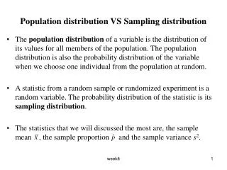
Terminology: • Parameter • A numerical descriptive measure of a population. • In statistical practice, the value of a parameter is not normally known. • Statistic • A numerical descriptive measure of a sample. • Use a statistic to estimate an unknown parameter.

parameter mean: μ standard deviation: σ proportion: p Sometimes we call the parameters “true”; true mean, true proportion, etc. statistic mean: x-bar standard deviation: s proportion: p-hat Sometimes we call the statistics “sample”; sample mean, sample proportion, etc. Compare

Notation:

Sampling Variability • When a sample is drawn at random from a given population, each sample drawn will be different. • These sample to sample differences are called sampling variability. • Sometimes, unfortunately, called sampling error, sampling variability is no error at all, but just the natural result of random sampling. • Sampling variability can be reduced by increasing the sample size.

Example: Sampling Variability • Frequency distribution for the number of accidents by bus drivers. • The population – 708 bus drivers employed by public corporations and the number of traffic accidents in which each bus driver was involved during a 4-year period. • Four different samples of 50 observations from this population. • The histograms of these five distributions (population and 4 samples) resemble one another in a general way, but there are obvious dissimilarities due to sampling variability.

The Population:

The Samples:

Sampling Distribution • Is a distribution of a sample statistic in all possible samples of the same size from the same population. • Note the “-ing” on the end of Sample. It looks and sounds similar to the Sample Distribution, but in reality the concept is much closer to a population model.

Continued • It is a model of a distribution of scores, like the population distribution, except that the scores are not raw scores, but statistics. • It is a thought experiment; “what would the world be like if a person repeatedly took samples of size N from the population distribution and computed a particular statistic each time?” • The resulting distribution of statistics is called the sampling distribution. • Every statistic has a sampling distribution.

Example: Sampling Distribution • Westvaco is laying off workers. There are 10 workers who could have been laid off; their ages are {25, 33, 35, 38, 48, 55, 55, 55, 56, 64}. • The ages of the three workers actually laid off were 55, 55, and 64. • Did Westvaco discriminate against the three laid off workers due to age?

Solution: • Randomly select three workers, without replacement because you can’t layoff the same worker twice, from the 10 possible for being laid off. • The summary statistic is the mean age of the three workers chosen at random. • Repeat this process many times in order to generate a sampling distribution of the summary statistic. • From this sampling distribution, make a decision about whether it was reasonable to assume that workers were selected for layoff without respect to their age.

The Sampling Distribution The actual mean age of the laid off workers was 58. As can be seen it is hard to get a mean age that large just by chance. Westvaco has some explaining to do.

Steps for Generating a Sampling Distribution • Random Sample – take a random sample of a fixed size n from the population (may be simulated). • Summary Statistic – Compute a summary statistic. • Repetition – Repeat steps 1 and 2 many times. • Distribution – display the distribution of the summary statistics.

Describing Sampling Distributions • Use the same tools of data analysis used to describe any distribution. • Overall shape • Outliers • Center • Spread

Example: • This sampling distribution is approximately normal, with a slight skew to the right, mean 7.31, standard deviation 2.39, and no outliers.

Bias of a Statistic • How well does a statistic estimate the value of a parameter. • Sampling distributions allow use to describe bias more precisely by speaking of the bias of a statistic rather than bias in a sampling method. • Bias concerns the center of the sampling distribution.

Unbiased Statistic/Unbiased Estimator • A statistic used to estimate a parameter is unbiased if the mean of its sampling distribution is equal to the true value of the parameter being estimated. • The statistic is then called an unbiased estimator of the parameter.

Example: Unbiased Statistic • The approximate sampling distributions for sample proportions for SRS’s of two sizes drawn from a population with p = 0.37. • (a) Sample size 100 (b) Sample size 1000 • Both statistics are unbiased because the means of the distributions equal the true population value p = 0.37. • The statistic from the larger sample is less variable.

Variability of a Statistic • Is described by the spread of its sampling distribution. • This spread is determined by the sampling design and the size of the sample. Larger samples give smaller spread. • As long as the population is much larger than the sample (at least 10 times as large), the spread of the sampling distribution is approximately the same for any population size.

Examples: Bias and Variability • Think of the true value of the population parameter as the bull’s-eye on a target. • Bias means our aim is off and we consistently miss the bull’s-eye in the same direction. Our sample values do not center on the population value. • Variability means how widely scattered our shots are on the target.

Determine Bias & Variability

Summary Bias and Variability

Hi Bias and Hi Variability Practice: State bias and variability

Low Bias and Low Variability Practice: State bias and variability

Low Bias and Hi Variability Practice: State bias and variability

Hi Bias and Low Variability Practice: State bias and variability

Sample Proportions

Sample Proportions • Rather than showing real repeated samples, imagine what would happen if we were to actually draw many samples. • Now imagine what would happen if we looked at the sample proportions for these samples. • The histogram we’d get if we could see all the proportions from all possible samples is called the sampling distribution of the proportions. • What would the histogram of all the sample proportions look like?

Sample Proportions • We would expect the histogram of the sample proportions to center at the true proportion, p, in the population. • As far as the shape of the histogram goes, we can simulate a bunch of random samples that we didn’t really draw. • It turns out that the histogram is unimodal, symmetric, and centered at p. • More specifically, it’s an amazing and fortunate fact that a Normal model is just the right one for the histogram of sample proportions.

Sample Proportion • The symbol for the sample proportion is (read as “p-hat”). • Example – Suppose your sample of 40 automobile drivers contains 26 who use seat belts. Then

Example • A Gallup Poll found that 210 out of a random sample of 501 American teens age 13 to 17 knew the answer to this question: • “What year did Columbus “discover” America?

Interpretation • The sample proportion is 210/501 =.42 • Is .42 a parameter or a statistic? • Does this mean that only 42% of American teens know this fact? • What is the proper notation for this statistic? • = .42

Modeling the Distribution of Sample Proportions • Modeling how sample proportions vary from sample to sample is one of the most powerful ideas we’ll see in this course. • A sampling distribution model for how a sample proportion varies from sample to sample allows us to quantify that variation and how likely it is that we’d observe a sample proportion in any particular interval. • To use a Normal model, we need to specify its mean and standard deviation. We’ll put µ, the mean of the Normal, at p.

Modeling the Distribution of Sample Proportions • When working with proportions, knowing the mean automatically gives us the standard deviation as well—the standard deviation we will use is • So, the distribution of the sample proportions is modeled with a probability model that is

Modeling the Distribution of Sample Proportions • A picture of the Distribution of Sample Proportions is as follows:

Characteristics of the Sampling Distribution of a Sample Proportion • The sampling distribution of is approximately normal and is closer to a normal distribution when the sample size n is large.

Continued: • The mean of the sampling distribution of is exactly p (the population parameter). • The standard deviation of the sampling distribution of is;

Summary: Sampling Distribution of a Sample Proportion

Formulas for Sampling Proportions

Sample Proportions – Sampling Variability • Because we have a Normal model, for example, we know that 95% of Normally distributed values are within two standard deviations of the mean. • So we should not be surprised if 95% of various polls gave results that were near the mean but varied above and below that by no more than two standard deviations. • This is what we mean by sampling error. It’s not really an error at all, but just variability you’d expect to see from one sample to another. A better term would be sampling variability.

Behavior of • Because the mean of the sampling distribution of is always equal to the parameter p, the sample proportion is an unbiased estimator of p. • The standard deviation of gets smaller as the sample size n increases because n is in the denominator of the formula for standard deviation. That is, is less variable in larger samples. • is less variable in larger samples.

How Good Is the Normal Model? • The Normal model gets better as a good model for the distribution of sample proportions as the sample size gets bigger. • Just how big of a sample do we need? This will soon be revealed…

Assumptions and Conditions • Most models are useful only when specific assumptions are true. • There are two assumptions in the case of the model for the distribution of sample proportions: • The Independence Assumption: The sampled values must be independent of each other. • The Sample Size Assumption: The sample size, n, must be large enough.

Assumptions and Conditions • Assumptions are hard—often impossible—to check. That’s why we assume them. • Still, we need to check whether the assumptions are reasonable by checking conditions that provide information about the assumptions. • The corresponding conditions to check before using the Normal model to model the distribution of sample proportions are the Randomization Condition, the 10% Condition and the Success/Failure Condition.

Sampling Distribution Models