Sampling Distribution Theory
Sampling Distribution Theory. ch6. Two independent R.V.s have the joint p.m.f. = the product of individual p.m.f.s. Ex6.1-1: X1is the number of spots on a fair die. f 1 (x 1 )=1/6, x 1 =1,2,3,4,5,6. X 2 is the number of heads on 4 indep. Tosses of a fair coin.


Sampling Distribution Theory
E N D
Presentation Transcript
Two independent R.V.s have the joint p.m.f. = the product of individual p.m.f.s. • Ex6.1-1: X1is the number of spots on a fair die. • f1(x1)=1/6, x1=1,2,3,4,5,6. • X2is the number of heads on 4 indep. Tosses of a fair coin. • If X1 and X2 are indep. • If X1 and X2 have the same p.m.f., their joint p.m.f. is f(x1)*f(x2). • This collection of X1and X2is a random sample of size n=2 from f(x). P(X1=1,2 & X2=3,4)
Linear Functions of Indep. R.V.s • Suppose a function Y=X1+X2, S1={1,2,3,4,5,6}, S2={0,1,2,3,4}. • Y will have the support S={1,2,…,9,10}. • The p.m.f. g(y) of Y is • The mathematical expectation (or expected value) of a function Y=u(X1,X2) is • If X1and X2 are indep.
Example • Ex6.1-2: X1 and X2 are two indep. R.V. from casting a die twice. • E(X1)=E(X2)=3.5; Var(X1)=Var(X2)=35/12; E(X1X2)=E(X1)E(X2)=12.25; • E[(X1-3.5)(X2-3.5)]=E(X1-3.5)E(X2-3.5)=0. • Y=X1+X2 →E(Y)= E(X1)+E(X2)=7; • Var(Y)=E[(X1+X2-7)2]=Var(X1)+Var(X2)=35/6. • The p.m.f. g(y) of Y with S={2,3,4,…,12} is
General Cases • If X1,…,Xn are indep., then their joint p.d.f. is f1(x1) …fn(xn). • The expected value of the product u1(x1) …un(xn) is the product of the expected values of u1(x1),…, un(xn). • If all these n distributions are the same, the collection of n indep. and identically distributed (iid) random variables, X1,…,Xn, is a random sample of size n from that common distribution. • Ex6.1-3: X1, X2, X3, are a random sample from a distribution with p.d.f. f(x)=e-x, 0<x<∞. • The joint p.d.f. is P(0 < X1 < 1,2 < X2 < 4,3 < X3 < 7)
Distributions of Sums of Indep. R.V.s • Distributions of the product of indep. R.V.s are straightforward. • However, distributions of the sum of indep. R.V.s are fetching: • First, the joint p.m.f. or p.d.f. is a simple product. • However, through summation, these R.V.s interfere with each other. • Care must be taken to distinguish some sum value happens more frequently than the others. • Sampling distribution theory is to derive the distributions of the functions of R.V.s (random variables). • The sample mean and variance are famous functions. • The summation of R.V.s is another example.
Example • Ex6.2-1: X1 and X2 are two indep. R.V.s from casting a 4-sided die twice. • The p.m.f. f(x)=, x=1,2,3,4. • The p.m.f. of Y=X1+X2 with S={2,3,4,5,6,7,8} is g(y): (convolution formula) g(2)= g(3)= g(y)=
Theorems • Thm6.2-1: X1,…,Xn are indep. and have the joint p.m.f. is f1(x1) …fn(xn). Y=u(X0,…,Xn) have the p.m.f. g(y) • Then if the summations exist. • For continuous type, integrals replace the summations. • Thm6.2-2: X1,…,Xn are indep. and their means exist, • Then, • Thm6.2-3: If X1,…,Xn are indep. with means μ1,…,μn and variances σ12,…,σn2, then Y=a1X1+…+anXn, where ai’s are real constants, have the mean and variance: • Ex6.2-3: X1 & X2 are indep. with μ1= -4, μ2=3 and σ12=4, σ22=9. • Y=3X1-2X2 has
Moment-generating Functions • Ex6.2-4: X1,…,Xn are a random sample of size n from a distribution with mean μand variance σ2; then • The sample mean: • Thm6.2-4: If X1,…,Xn are indep. R.V.s with moment-generating functions , i=1..n, then Y=a1X1+…+anXn, has the moment-generating • Cly6.2-1: If X1,…,Xn are indep. R.V.s with M(t), • then Y=X1+…+Xn has MY(t)=[M(t)]n. • has MY(t)
Examples • Ex6.2-5: X1,…,Xn are the outcomes on n Bernoulli trials. • The moment-generating function of Xi, i=1..n, is M(t)=q+pet. • Then Y=X1+…+Xn has MY(t)=[q+pet]n, which is b(n,p). • Ex6.2-6: X1,X2,X3 are the outcomes of a random sample of size n=3 from the exponential distribution with mean θand M(t)=1/(1-θt), t<1/θ. • Then Y=X1+X2+X3 has MY(t)=[1/(1-θt)]3=(1-θt)-3,which is a gamma distribution with α=3, and θ. • has a gamma distribution with α=3, and θ/3.
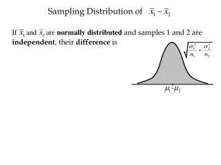
Statistics on Normal Distributions • Thm6.3-1: X1,…,Xn are the outcomes on a random sample of size n from the normal distribution N(μ,σ2). • The distribution of the sample mean is N(μ,σ2/n). • Pf: • Thm6.3-2: X1,…,Xn are independent and have χ2(r1),…, χ2(rn) distributions, respectively ; Then, Y=X1+…+Xn is χ2(r1+…+rn). • Pf: • Thm6.3-3: Z1,…,Zn are independent and all have N(0,1); Then, W=Z12+…+Zn2is χ2(n). Pf: Thm4.4-2: If X is N(μ,σ2), then V=[(X-μ)/σ]2=Z2 is χ2(1).Thm6.3-2: Y=X1+…+Xn is χ2(r1+…+rn)= χ2(n) in this case. MX(t) MY(t)=
Example • Fig.6.3-1: p.d.f.s of means of samples from N(50,16). • is N(50, 16/n).
Theoretical Mean and Sample Mean • Cly6.3-1: Z1,…,Zn are independent and have N(μi,σi2),i=1..n; Then, W=[(Z1-μ1)/σi2]2+…+[(Zn-μn)/σn2]2 is χ2(n). • Thm6.3-4: X1,…,Xn are the outcomes on a random sample of size n from the normal distribution N(μ,σ2). Then, • The sample mean & variance are indep. • is χ2(n-1) Pf: (a) omitted; (b): As theoretical mean is replaced by the sample mean, one degree of freedom is lost! MV(t)
Linear Combinations of N(μ,σ2) • Ex6.3-2: X1,X2,X3,X4 are a random sample of size 4 from the normal distribution N(76.4,383). Then P(0.711W 7.779)=0.9-0.05=0.85, P(0.352 V 6.251)=0.9-0.05=0.85 • Thm6.3-5: If X1,…,Xn are n mutually indep. normal variables with means μ1,…,μn & variances σ12,…,σn2, then the linear function has the normal distribution Pf: By moment-generating function, … • Ex6.3-3: X1:N(693.2,22820) and X2:N(631.7,19205) are indep. Find P(X1>X2) • Y=X1-X2 is N(61.5,42025). • P(X1>X2)=P(Y>0)=
Central Limit Theorem • Ex6.2-4: X1,…,Xn are a random sample of size n from a distribution with mean μand variance σ2; then The sample mean: • Thm6.4-1: (Central Limit Theorem) If is the mean of a random sample X1,…,Xn of size n from some distribution with a finite mean μand a finite positive variance σ2, then the distribution of is N(0, 1) in the limit as n →∞. Even if Xi is not N(μ,σ2). if n is large W= W
More Examples • Ex6.4-1: Let denote the mean of a random sample of size n=15 from the distribution whose p.d.f. is f(x)=3x2/2, -1<x<1. • μ=0, σ2=3/5. • Ex6.4-2: Let X1,…,X20 be a random sample of size 20 from the uniform distribution U(0,1). • μ=½, σ2=1/12; Y=X1+…+X20. • Ex6.4-3: Let denote the mean of a random sample of size n=25 from the distribution whose p.d.f. is f(x)=x3/4, 0<x<2 • μ=1.6, σ2=8/75.
How large of size n is sufficient? • If n=25, 30 or larger, the approximation is generally good. • If the original distribution is symmetric, unimodal and of continuous type, n can be as small as 4 or 5. • If the original is like normal, n can be lowered to 2 or 3. • If it is exactly normal, n=1 or more is just good. • However, if the original is highly skew, n must be quite large. • Ex6.4-4: Let X1,…,X4 be a random sample of size 4 from the uniform distribution U(0,1) with p.d.f. f(x)=1, 0<x<1. • μ=½, σ2=1/12; Y=X1+X2.Y=X1+…+X4.
Graphic Illustration • Fig.6.4-1: Sum of n U(0, 1) R.V.s N( n(1/2), n(1/12) ) p.d.f.
Skew Distributions • Suppose f(x) and F(x) are the p.d.f. and distribution function of a random variable X with mean μ and variance σ2. • Ex6.4-5: Let X1,…,Xn be a random sample of size n from a chi-square distribution χ2(1). • Y=X1+…+Xn is χ2(n), E(Y)=n, Var(Y)=2n. n=20 or 100 →N( , ).
Graphic Illustration • Fig.6.4-2: The p.d.f.s of sums of χ2(1), transformed so that their mean is equal to zero and variance is equal to one, becomes closer to the N(0, 1) as the number of degrees of freedom increases.
Simulation of R.V. X with f(x) & F(x) • Random number generator will produce values y’s for U(0,1). • Since F(x)=U(0,1)=Y, x=F-1(y) is an observed or simulated value of X. • Ex.6.4-6: Let X1,…,Xn be a random sample of size n from the distribution with f(x), F(x), mean μand variance σ2. • 1000 random samples are simulated to compute the values of W. • A histogram of these values are grouped into 21 classes of equal width. f(x)=(x+1)/2, F(x)=(x+1)2/4, f(x)=3x2/2, F(x)=(x3+1)/2, -1<x<1; μ=1/3, σ2=2/9. -1<x<1; μ=0, σ2=3/5. N(0,1)
Approximation of Discrete Distributions • Let X1,…,Xn be a random sample from a Bernoulli distribution with μ=p and σ2=npq, 0<p<1. • Thus, Y=X1+…+Xn is binomial b(n,p). →N(np,npq) as n →∞. • Rule: n is “sufficiently large” if np5 and nq5. • If p deviates from 0.5 (skew!!), n need to be larger. • Ex.6.5-1: Y, b(10,1/2), can be approximated by N(5,2.5). • Ex.6.5-2: Y, b(18,1/6), can be hardly approx. by N(3,2.5), ∵3<5.
Another Example • Ex6.5-4: Y is b(36,1/2). • Correct Probability: • Approximation of Binomial Distribution b(n,p): Good approx.!
Approximation of Poisson Distribution • Approximation of a Poisson Distribution Y with mean λ: • Ex6.5-5: X that has a Poisson distribution with mean 20 can be seen as the sum Y of the observations of a random sample of size 20 from a Poisson distribution with mean 1. • Correct Probability: Fig.6.5-3: Normal approx. of the Poisson Probability Histogram
Student’s T Distribution • Gossett, William Sealy published “t-test” in Biometrika1908 to measure the confidence interval, the deviation of “small samples” from the “real”. • Suppose the underlying distribution is normal with unknown σ2. • Fig.6.6-1(a): The T p.d.f. becomes closer to the N(0, 1) p.d.f. as the number of degrees of freedom increases. tα(r) is the 100(1-α) percentile, or the upper 100αpercent point. [Table VI, p.658] f(t)= Onlydepends on r!
Examples • Ex6.6-1: Suppose T has a t distribution with r=7. • From Table VI on p.658, • Ex6.6-2: Suppose T has a t distribution with r=14. • Find a constant c, such that P(|T|<c)=0.9 • From Table VI on p.658,
F Distribution: F(r1, r2) • From two indep. random samples of size n1 & n2 from N(μ1,σ12) & N(μ2,σ22),some comparisons can be performed, such as: • Fα(r1,r2)is the upper 100α percent point. [Table VII, p.659~663] • Ex6.6-4: Suppose F has a F(4,9) distribution. • Find constants c & d, such that P(F c)=0.01, P(F d)=0.05 c=F0.99(4,9) If F is F(6,9):