Download
1 / 26
440 likes | 2.26k Views
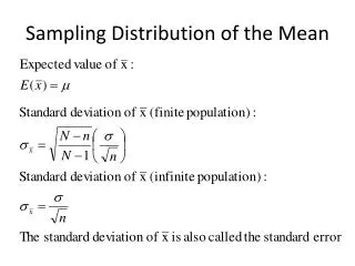
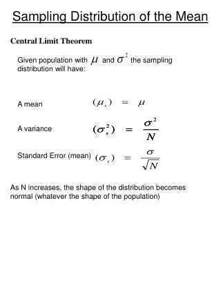
Central Limit Theorem. Sampling Distribution of the Mean. Given population with and the sampling distribution will have:. A mean. A variance. Standard Error (mean). As N increases, the shape of the distribution becomes normal (whatever the shape of the population).

E N D
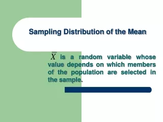
Central Limit Theorem Sampling Distribution of the Mean Given population with and the sampling distribution will have: A mean A variance Standard Error (mean) As N increases, the shape of the distribution becomes normal (whatever the shape of the population)
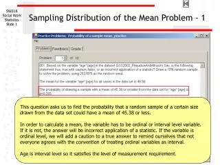
Testing Hypothesis Known and Remember: We could test a hypothesis concerning a population and a single score by Obtain and use z table We will continue the same logic Given: Behavior Problem Score of 10 years olds Sample of 10 year olds under stress Because we know and , we can use the Central Limit Theorem to obtain the Sampling Distribution when H0 is true.
Sampling Distribution will have We can find areas under the distribution by referring to Z table We need to know Minor change from z score NOW or With our data Changes in formula because we are dealing with distribution of means NOT individual scores.
From Z table we find is 0.0901 Because we want a two-tailed test we double 0.0901 (2)0.0901 = 0.1802 NOT REJECT H0 or is
One-Sample t test Pop’n = known & unknown we must estimate with Because we use S, we can no longer declare the answer to be a Z, now it is a t Why? Sampling Distribution of t - S2 is unbiased estimator of - The problem is the shape of the S2 distribution positively skewed
thus: S2 is more likely to UNDERESTIMATE (especially with small N) thus: t is likely to be larger than Z (S2 is in denominator) t - statistic and substitute S2 for To treat t as a Z would give us too many significant results
Guinness Brewing Company (student) Student’s t distribution we switch to the t Table when we use S2 Go to Table Unlike Z, distribution is a function of with Degrees of Freedom For one-sample cases, lost because we used (sample mean) to calculate S2 all x can vary save for 1
Example: One-Sample Unknown Effect of statistic tutorials: (no tutorials) Last 100 years: (tutorials) this years: N = 20, S = 6.4
Go to t-Table t-Table - not area (p) above or below value of t - gives t values that cut off critical areas, e.g., 0.05 - t also defined for each df N=20 df = (N-1) = 20-1 = 19 Go to Table t.05(19) is 2.093 critical value reject
Factors Affecting Magnitude of t & Decision 1. Difference between and the larger the numerator, the larger the t value 2. Size of S2 as S2 decreases, t increases 3. Size of N as N increases, denominator decreases, t increases 4. level 5. One-, or two-tailed test
Confidence Limits on Mean Point estimate Specific value taken as estimator of a parameter Interval estimates A range of values estimated to include parameter Confidence limits Range of values that has a specific (p) of bracketing the parameter. End Points = confidence limits. How large or small could be without rejecting if we ran a t-test on the obtained sample mean.
Confidence Limits (C.I.) We already know , S and We know critical value for t at We solve for Rearranging Using +2.993 and -2.993
Two Related Samples t Related Samples Design in which the same subject is observed under more than one condition (repeated measures, matched samples) Each subject will have 2 measures and that will be correlated. This must be taken into account. Promoting social skills in adolescents Before and after intervention before after Difference Scores Set of scores representing the difference between the subject’s performance or two occasions
our data can be the D column from we are testing a hypothesis using ONE sample
Related Samples t remember now N = # of D scores Degrees of Freedom same as for one-sample case = (N - 1) = (15 - 1) = 14 our data Go to table
Advantages of Related Samples 1. Avoids problems that come with subject to subject variability. The difference between(x1) 26 and (x2) 24 is the same as between (x1) 6 and (x2) 4 (increases power) (less variance, lower denominator, greater t) 2. Control of extraneous variables 3. Requires fewer subjects Disadvantages 1. Order effects 2. Carry-over effects
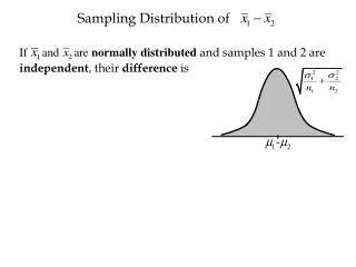
Two Independent Samples t Sampling distribution of differences between means Suppose: 2 pop’ns and and and draw pairs of samples: sizes N1, and N2 record means and and the differences between , and for each pair of samples repeat times
Mean Difference Mean Variance Standard Error Variance Sum Law Variance of a sum or difference of two INDEPENDENT variables = sum of their variances The distribution of the differences is also normal
t Difference Between Means We must estimate with Because or
is O.K. only when the N’s are the same size When we need a better estimate of We must assume homogeneity of variance Rather than using or to estimate , we use their average. Because we need a Weighted Average weighted by their degrees of freedom Pooled Variance
Now come from formula for Standard Error Degrees of Freedom two means have been used to calculate
Example: We have numerator 18.00 – 15.25 We need denominator ??????? Pooled Variance because Denominator becomes =
Summary If and are known, then treat as in Z score formula; replaces If is known and is unknown, then replaces in If two related samples, then replaces and replaces
If two independent samples, and Ns are of equal size, then is replaced by If two independent samples, and Ns are NOT equal, then and are replaced by