Download
1 / 1
10 likes | 128 Views
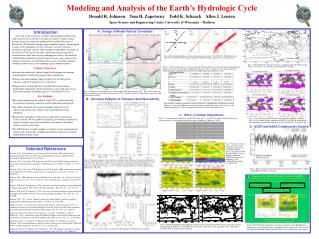
Modeling and Analysis of the Earth’s Hydrologic Cycle Donald R. Johnson Tom H. Zapotocny Todd K. Schaack Allen J. Lenzen Space Science and Engineering Center, University of Wisconsin – Madison. Field. Observed. UW model. All sky OLR (W m -2 ). 234.8. 238.4.

E N D
Modeling and Analysis of the Earth’s Hydrologic Cycle Donald R. Johnson Tom H. Zapotocny Todd K. Schaack Allen J. Lenzen Space Science and Engineering Center, University of Wisconsin – Madison Field Observed UW model All sky OLR (W m-2) 234.8 238.4 Clear sky OLR (W m-2) 264.0 266.3 Total cloud forcing (W m-2) -19.0 -13.4 Longwave cloud forcing (W m-2) 29.2 27.9 Shortwave cloud forcing (W m-2) -48.2 -41.3 Total Cloud fraction (%) 52.2 to 62.5 60.7 Precipitable water (mm) 24.7 22.8 Precipitation (mm day-1) 2.7 3.1 Latent heat flux (W m-2) 78.0 89.9 Sensible heat flux (W m-2) 24.0 16.3 Introduction A. Design of Model Vertical Coordinate A Day 10 UW B Day 10 UW C Day 10 CCM3 • A key aim of this research is to further understanding of global water vapor and inert trace constituent transport in relation to climate change through analysis of simulations produced by the global University of Wisconsin (UW) hybrid isentropic-sigma coordinate models. Advancing the accuracy of the simulation of water substances, aerosols, chemical constituents, potential vorticity and stratospheric-tropospheric exchange are all critical to DOE’s goal of accurate climate prediction on decadal tocentennial time scales and assessing anthropogenic effects. Research has established that simulations of the transport of water vapor, and inert and chemical constituents are remarkably more accurate in hybrid isentropic coordinate models than in corresponding sigma coordinate models. • Primary Objectives: • Advance the modeling of climate change by developing an isentropic hybrid model for global and regional climate simulations. • Advance the understanding of physical processes involving water substances and the transport of trace constituents. • Diagnostically examine the limits of global and regional climate predictability imposed by inherent limitations in the simulation of trace constituent transport, hydrologic processes and cloud life-cycles. Key Findings: • The results demonstrate the viability of the UW model for long term climate integration, numerical weather prediction and chemistry. • The studies document that no insurmountable barriers exist for realistic simulations of the climate state with the hybrid vertical coordinate. • Experiments reported here demonstrate a high degree of numerical accuracy for the UW model in simulating reversibility and potential vorticity transport over 10 day period that corresponds to the global residence time of water vapor. • The UW hybrid model simulates seasonally varying and interannual climate scales realistically, including monsoonal circulations associated with El Nino/La Nina events. Fig. 4. Bivariate distributions of ozone and a proxy trace ozone. The “Day 10” distributions from the UW model, UW model, and T42 CCM3 are shown in panels (A)-(C) respectively. Fig. 7. The distribution of annual vertically averaged heating (10-1 K/Day) from the last 13 years of a 14 year climate runwithUW model. Table 1. Results from analysis of variance globally for the difference of equivalent potential temperature minus its trace (e-t e) and three components at day 10. Units of variance are the square of Kelvin temperature (K2). Quantity in parenthesis is the RMS temperature difference (±K). Fig. 1. Schematic of meridional cross sections along 104E for 05 August 1981. The red lines represent potential temperature; the black lines represent UW model surfaces; the green lines represent scaled sigma model surfaces. B. Accuracy Analysis of Transport and Reversibility A. UW model along 24S CI=2 K B. UW model along 59S CI=2 K The first three columns respectively list the variances of 1) the differences about the area mean difference, 2) area mean differences about the grand mean difference and 3) the variance of the grand mean difference. The last column lists the total variance of the differences. C. UW Climate Simulations Table 2. A comparison of annually averaged fields from the 13-year UW model climate simulation to observed values. Observational estimates are from a summary by Hack et al. 1998. Fig. 8. The time averaged distributions of precipitation (mm/day) from the 13 year UW model climate simulation for DJF (A) and JJA (B) and from the Xie and Arkin precipitation climatology for 1979-99 for DJF (C) and JJA (D). D. NCEP and NASA Collaborative Studies A B Fig. 5. The time averaged mean sea-level pressure distributions from the 13 year UW model climate simulation for DJF (A) and JJA (B) as well as differences from the NCEP/NCAR reanalysis climatology (UW-NCEP/NCAR) for DJF (C) and JJA (D). Selected References Schaack, T. K., T. H. Zapotocny, A. J. Lenzen and D. R. Johnson, 2004: Global climate simulation with the University of Wisconsin global hybrid isentropic coordinate model. Accepted for publication in Journal of Climate. Johnson, D. R., A. J. Lenzen, T. H. Zapotocny and T. K. Schaack, 2002: Entropy, numerical uncertainties and modeling of atmospheric hydrologic processes: Part B. J. Climate, 15, 1777-1804. Johnson, D. R., A. J. Lenzen, T. H. Zapotocny, and T. K. Schaack, 2000: Numerical uncertainties in the simulation of reversible isentropic processes and entropy conservation. J. Climate, 13, 3860-3884. Johnson, D. R., 2000: Entropy, the Lorenz Energy Cycle and Climate. In “General Circulation Model Development: Past, Present and Future” (D. A. Randall, ed.), Academic Press, pp. 659-720. Reames, F. M. and T. H. Zapotocny, 1999a: Inert trace constituent transport in sigma and hybrid isentropic-sigma models. Part I: Nine advection algorithms. Mon. Wea. Rev., 127, 173-187. Reames, F. M. and T. H. Zapotocny, 1999b: Inert trace constituent transport in sigma and hybrid isentropic-sigma models. Part II: Twelve semi-Lagrangian algorithms. Mon. Wea. Rev., 127, 188-200. Johnson, D. R., 1997: On the "General Coldness of Climate Models" and the Second Law: Implications for Modeling the Earth System. J. Climate, 10, 2826-2846. Zapotocny, T. H., A. J. Lenzen, D. R. Johnson, F. M. Reames, and T. K. Schaack, 1997a: A comparison of inert trace constituent transport between the University of Wisconsin isentropic-sigma model and the NCAR community climate model. Mon. Wea. Rev., 125, 120-142. Zapotocny, T. H., D. R. Johnson, T. K. Schaack, A. J. Lenzen, F. M. Reames, and P. A. Politowicz, 1997b: Simulations of Joint Distributions of Equivalent Potential Temperature and an Inert Trace Constituent in the UW Model and CCM2. Geophys. Res. Let., 24, 865-868. Zapotocny, T. H., A. J. Lenzen, D. R. Johnson, F. M. Reames, P. A. Politowicz, and T. K. Schaack, 1996: Joint distributions of potential vorticity and inert trace constituent in CCM2 and UW model simulations. Geophys. Res. Let., 23, 2525-2528. Zapotocny, T. H., D. R. Johnson, and F. M. Reames, 1994: Development and initial test of the University of Wisconsin global isentropic-sigma model. Mon. Wea. Rev., 122, 2160-2178. Fig. 2. The top two panels show zonal cross sections of the difference between e and trace e (CI=2 K) from the UW model at day 10.Panel C shows a bivariate distribution ofe and trace e at day 10, panel D shows a relative frequency distribution of simulated differences between e and trace e at days 2.5, 5, 7.5 and 10, and panel E shows a vertical profile of the differences at day 10. C D Fig. 9. Fifteen month record of Anomaly Correlation from the UW model and NCEP Global Forecast System. A NI A B Fig. 6. Global distributions of the difference (DJF 1987-88 minus DJF 1988-89) between seasonally average precipitation for DJF 1987-88 and DJF 1988-89 (mm/day) from the (A) Xie and Arkin (1997) climatology and (B) UW model climate simulation. Fig 10. The UW hybrid model forms the global component of the RAQMS data assimilation system. Figure B shows tropospheric ozone burden (DU) for June-July 1999 from the RAQMS assimilation while Fig. A is the satellite observed estimate. Fig. 3. Same as Fig. 2 except for CCM3 running at T42 horizontal resolution.