Statistics & Flood Frequency Chapter 3
500 likes | 771 Views
Statistics & Flood Frequency Chapter 3. Dr. Philip B. Bedient Rice University 2006. Predicting FLOODS. Flood Frequency Analysis. Statistical Methods to evaluate probability exceeding a particular outcome - P (X >20,000 cfs) = 10% Used to determine return periods of rainfall or flows

Statistics & Flood Frequency Chapter 3
E N D
Presentation Transcript
Statistics & Flood FrequencyChapter 3 Dr. Philip B. Bedient Rice University 2006
Flood Frequency Analysis • Statistical Methods to evaluate probability exceeding a particular outcome - P (X >20,000 cfs) = 10% • Used to determine return periods of rainfall or flows • Used to determine specific frequency flows for floodplain mapping purposes (10, 25, 50, 100 yr) • Used for datasets that have no obvious trends • Used to statistically extend data sets
Random Variables • Parameter that cannot be predicted with certainty • Outcome of a random or uncertain process - flipping a coin or picking out a card from deck • Can be discrete or continuous • Data are usually discrete or quantized • Usually easier to apply continuous distribution to discrete data that has been organized into bins
Typical CDF Continuous F(x1) - F(x2) Discrete F(x1) = P(x < x1)
Frequency Histogram 36 27 17.3 1.3 9 1.3 8 Probability that Q is 10,000 to 15, 000 = 17.3% Prob that Q < 20,000 = 1.3 + 17.3 + 36 = 54.6%
Probability Distributions CDF is the most useful form for analysis
Moments of a Distribution First Moment about the Origin Discrete Continuous
Estimates of Moments from Data Std Dev.Sx = (Sx2)1/2
Skewness CoefficientUsed to evaluate high or low data points - flood or drought data
Mean, Median, Mode • Positive Skew moves mean to right • Negative Skew moves mean to left • Normal Dist’n has mean = median = mode • Median has highest prob. of occurrence
01 76 83 '98
Siletz River Data Stationary Data Showing No Obvious Trends
Frequency Histogram 36 27 17.3 1.3 9 1.3 8 Probability that Q is 10,000 to 15, 000 = 17.3% Prob that Q < 20,000 = 1.3 + 17.3 + 36 = 54.6%
Cumulative Histogram Probability that Q < 20,000 is 54.6 % Probability that Q > 25,000 is 19 %
Major Distributions • Binomial - P (x successes in n trials) • Exponential - decays rapidly to low probability - event arrival times • Normal- Symmetric based on m and s • Lognormal - Log data are normally dist’d • Gamma - skewed distribution - hydro data • Log Pearson III -skewed logs -recommended by the IAC on water data - most often used
Binomial Distribution The probability of getting x successes followed by n-x failures is the product of prob of n independent events: px (1-p)n-x This represents only one possible outcome. The number of ways of choosing x successes out of n events is the binomial coeff. The resulting distribution is the Binomial or B(n,p). Bin. Coeff for single success in 3 years = 3(2)(1) / 2(1) = 3
Risk and Reliability • The probability of at least one success in n years, where the probability of success in any year is 1/T, • is called the RISK. • Prob success = p = 1/T and Prob failure = 1-p • RISK = 1 - P(0) • = 1 - Prob(no success in n years) • = 1 - (1-p)n • = 1 - (1 - 1/T)n • Reliability = (1 - 1/T)n
Design Periods vs RISK and Design Life Expected Design Life (Years) x 2 x 3
Risk Example What is the probabilityof at least one 50 yr flood in a 30 year mortgage period, where the probability of success in any year is 1/T = 1.50 = 0.02 RISK = 1 - (1 - 1/T)n = 1 - (1 - 0.02)30 = 1 - (0.98)30 = 0.455 or 46% If this is too large a risk, then increase design level to the 100 year where p = 0.01 RISK = 1 - (0.99)30 = 0.26 or 26%
Exponential Dist’n Poisson Process where k is average no. of events per time and 1/k is the average time between arrivals f(t) = k e - kt for t > 0 Traffic flow Flood arrivals Telephone calls
Exponential Dist’n f(t) = k e - kt for t > 0 F(t) = 1 - e - kt Avg Time Between Events
Gamma Dist’n Unit Hydrographs n =1 n =2 n =3
Normal, LogN, LPIII Data in bins Normal
Normal Prob Paper Normal Prob Paper converts the Normal CDF S curve into a straight line on a prob scale
Normal Prob Paper Std Dev = +1000 cfs Mean = 5200 cfs • Place mean at F = 50% • Place one Sx at 15.9 and 84.1% • Connect points with st. line • Plot data with plotting position formula P = m/n+1 Std Dev = –1000 cfs
Normal Dist’n Fit Mean
Frequency Analysis of Peak Flow Data • Take Mean and Variance (S.D.) of ranked data • Take Skewness Cs of data (3rd moment about mean) • If Cs near zero, assume normal dist’n • If Cs large, convert Y = Log x - (Mean and Var of Y) • Take Skewness of Log data - Cs(Y) • If Cs near zero, then fits Lognormal • If Cs not zero, fit data to Log Pearson III
Siletz River Example 75 data points - Excel Tools Original Q Y = Log Q
Siletz River Example - Fit Normal and LogN • Normal DistributionQ = Qm + z SQ • Q100 = 20452 + 2.326(6089) = 34,620 cfs • Mean + z (S.D.) • Where z = std normal variate - tables Log N Distribution Y = Ym + k SY Y100 = 4.29209 + 2.326(0.129) = 4.5923 k = freq factor and Q = 10Y = 39,100 cfs
Log Pearson Type III Log Pearson Type IIIY = Ym + k SY K is a function of Cs and Recurrence Interval Table 3.4 lists values for pos and neg skews For Cs = -0.15, thus K = 2.15 from Table 3.4 Y100 = 4.29209 + 2.15(0.129) = 4.567 Q = 10Y = 36,927 cfs for LP III Plot several points on Log Prob paper
LogN Prob Paper for CDF • What is the prob that flow exceeds some given value - 100 yr value • Plot data with plotting position formula P = m/n+1 , m = rank, n = # • Log N dist’n plots as straight line
LogN Plot of Siletz R. Mean Straight Line Fits Data Well
Siletz River Flow Data Various Fits of CDFs LP3 has curvature LN is straight line
Trends in data have to be removed before any Frequency Analysis 01 92 '98 98