Download
1 / 50
500 likes | 631 Views
Physics of the Atmosphere Physik der Atmosphäre. WS 2010 Ulrich Platt Institut f. Umweltphysik R. 424 Ulrich.Platt@iup.uni-heidelberg.de. Last Week.

E N D
Physics of the Atmosphere Physik der Atmosphäre WS 2010 Ulrich Platt Institut f. Umweltphysik R. 424 Ulrich.Platt@iup.uni-heidelberg.de
Last Week The „oxygen only“ chemistry of the „Chapman Cycle“ gives a good semi-quantitative explanation of the ozone layer (and an analytical expression of the O3 concentration as a function of altitude) A closer look reveals that actually strat. ozone levels are about a factor of 3 smaller than predicted by Chapman chemistry A series of reactions involving HOX, NOX, CLOX ,and BrOX chemistry catalyse the O+O3 2O2reaction and thus bring theory and observation in agreement.
Catalytic Ozone Destruction in the Stratosphere X + O3 XO + O2 XO + O X + O2 net: O + O3 2O2 X/XO: „catalyst“ (e.g. OH/HO2, NO/NO2, Cl/ClO, Br/BrO) HOX (Bates and Nicolet, 1950) NOX (Crutzen, 1970) ClOX (Stolarski and Cicerone, 1974; Molina and Rowland, 1974) Catalytic desctruction cyclesexplain difference between measured and calculated O3 profiles
Primary Sources of Chlorine for the Stratosphere (1999) From: Scientific Assessment of Ozone Depletion 2002, Fig. Q7-1, D. Fahey
Chlorine Chemistry in the Stratosphere Mid-latitude (unperturbed) stratosphere: ClONO2: 20%HCl: 80%ClO 1%
Vertical Profiles of CFC-11 and CFC-12 Altitude profiles of CFC-11 (bottom) and CFC-12 (top) [NASA, 1994].
Measurement of Chlorine Gases From Space (Nov. 1994, 35o-49oN) From: Scientific Assessment of Ozone Depletion 2002, Table Q8-2, D. Fahey
Vertical Profiles of Chlorine Source Gases (CFC's), Reservoir Species (HCl, ClONO2), and Reactive Species (Cl, ClO, …) in the Stratosphere
Atmospheric lifetimes, emissions,and Ozone Depletion Potentials of halogensource gases. From: Scientific Assessment of Ozone Depletion 2002, Table Q7-1, D. Fahey
Relevant Bromine Catalysed O3-Destruction Cycles a) BrO + O Br + O2 (2.52) Br + O3 BrO + O2Net: O + O3 2O2 b) BrO + BrO Br + Br + O2 (2.53) 2(Br + O3 BrO + O2) (2.54)Net: 2O3 3O2 The BrO-BrO self reaction leads also to the products Br2 + O2. Br2 can be photolysed to 2Br which also closes the cycle. c) BrO + ClO Br + ClOO (2.55) ClOO + M Cl + M + O2 (2.56) Cl + O3 ClO + O2 (2.57)Net: 2O3 3O2 The BrO-ClO reaction (McElroy mechanism) also leads to the products: Br + OClO (30%) (2.55b) BrCl + O2 (10%) (2.55c)
Primary Sources of Bromine for the Stratosphere (1999) From: Scientific Assessment of Ozone Depletion 2002, Fig. Q7-1, D. Fahey
Measured Stratospheric BrO Profiles Comparison of measured BrO profiles by different measurement techniques retrieved under different geophysical conditions at different times [Harder et al. 1998]. Also two model profiles [Chipperfield, 1999] are shown for the balloon-borne DOAS measurement flights at León (Spain) in Nov. 1996 and at Kiruna (North-Sweden) in Feb. 1997. From: Pfeilsticker et al.
Temporal evolution of daytime ClO 1991-1997 Temporal evolution of daytime ClO as measured by MLS (triangles) and modelled by SLIMCAT (solid line) at 4.6 hPa (36 km). The straight lines represent the linear trend fitted to the two data sets [Ricaud et al., 1997].
Stratospheric Cl-Burden 1960-2080 Predicted future atmospheric burden of chlorine (adapted from Brasseur [1995]).
Evolution of Global, Total Ozone Deseasonalized, area-weighted seasonal (3-month average) total ozone deviations, estimated from five different global datasets. Each dataset was deseasonalized with respect to the period 1979-1987, and deviations are expressed as percentages of the ground-based time average for the period 1964-1980. Results are shown for the region 60°S-60°N (top) and the entire globe (90°S-90°N) (bottom). The different satellite datasets cover 1979-2001, and the ground-based data extend back to 1964. TOMS, Total Ozone Mapping Spectrometer; SBUV, Solar Backscatter Ultraviolet; NIWA, National Institute of Water and Atmospheric Research (New Zealand). Adapted from Fioletov et al. (2002). From: Scientific Assessment of Ozone Depletion 2002, Figure 4-2
Evolution of Mid-Latitude (35o-60o) Total Ozone Deseasonalized, area-weighted total ozone deviations for the midlatitude regions of 35°N-60°N (top) and 35°S-60°S (bottom) (as in Figure 4-6), but smoothed by four passes of a 13-point running mean. Adapted from Fioletov et al. (2002). From: Scientific Assessment of Ozone Depletion 2002, Figure 4-7
The Global Ozone Trend Meridional cross section of ozone profile trends derived from the combined SAGE I (1979-1981) and SAGE II (1984-2000) datasets. Trends were calculated in percent per decade, relative to the overall time average. Shading indicates that the trends are statistically insignificant at the 2s (95%) level. Updated from H.J. Wang et al. (2002).From: Scientific Assessment of Ozone Depletion 2002, Fig. 4-9
Stratospheric Aerosol 1976-2000 Multiyear time series of stratospheric aerosols measured by lidar (694.3 nm) at Garmisch (47.5°N, 11.1°E) in Southern Germany (red curve) and zonally averaged SAGE II stratospheric aerosol optical depth (1020 nm) in the latitude band 40°N-50°N (black curve). Vertical arrows show major volcanic eruptions. Lidar data are given as particle backscatter integrated from 1 km above the tropopause to the top of the aerosol layer. The curve referring to SAGE II data was calculated as optical depth divided by 40. For reference, the 1979 level is shown as a dashed line. Data from Garmisch provided courtesy of H. Jäger (IFU, Germany). From: Scientific Assessment of Ozone Depletion 2002, Fig. 4-18
Global Ozone, Volcanic Eruptions,and the Solar Cycle From: Scientific Assessment of Ozone Depletion 2002, Fig. Q14-1, D. Fahey
One of the first observations of the Ozone Hole Observations of total ozone at Halley, Antarctica [Farman et al., 1986; Jones and Shanklin, 1995].
The Antarctic Ozone Hole in 1986 and 1997 Comparison of Ozone profiles at the South Pole for the month of October in different years. The ozone concentrations of the late 1960s and early 1970 are much higher than those of 1986 and 1997 [Solomon, 1998].
Ozone - ClO in the Antarctic 1987(Airborne Antarctic Ozone Expedition)
AAOE – Jim Anderson in situ instruments that have been designed, built, tested, and calibrated, and flown on NASA research aircraft, either the ER-2 or WB57-F. The instrument that measures members of the halogen family of molecules. The current instrument measures ClONO2 (Chlorine Nitrate), ClOOCl, ClO dimer, ClO, as well as NO2. Its earliest version was built and first flown in 1987 in the left wing pod of the NASA ER-2 aircraft to help determine the cause of ozone loss over Antarctica. [There could either be a discussion here of that effort or a link to that effort, with a list of the alternate mechanisms hypothesized for the formation of the ozone hole, and the politically charged atmosphere surrounding the mission.] The picture below illustrates simultaneous measurements of ClO and Ozone taken over Antarctica on August 23, 1987 and on September 16, 1987, before after significant ozone depletion has occurred. The clear anticorrelation exhibited in the second panel between ozone and ClO as the aircraft crosses into the Antarctic vortex illustrates the direct relationship between the presence of chlorine free radical and ozone depletion. The difference between the two panels is indicative of the time necessary for ozone to be removed by chlorine atoms formed from the photolysis of Cl2 produced on the surface of polar stratospheric clouds. This photolysis occurs quickly once the sun returns to the Antarctic lower stratosphere.
The Antarctic Ozone Hole 2001 From: Scientific Assessment of Ozone Depletion 2002, Fig. Q11-1, D. Fahey
Average Total Ozone in Polar Regions From: Scientific Assessment of Ozone Depletion 2002, Fig. Q11-1, D. Fahey
Polar Stratospheric Clouds Schematic drawing of the dynamic and photochemical evolution of the stratosphere during polar winter/spring.
Under these conditions the stratospheric chemistry changes substantially: In the darkness of the polar night NOx is converted into N2O5 NO2 + O3 NO3 (2.58) NO2 + NO3 N2O5 (2.59) N2O5 is then converted into HNO3 (see below); these processes are referred to as denoxification. The cold vortex temperatures are the prerequisite for the formation of polar stratospheric clouds (PSCs). Reactions not possible in the gas phase occur on the surfaces of those PSC particles: ClONO2 (g) + HCl (s) HNO3 (s) + Cl2 (g) (2.60) ClONO2 (g) + H2O (s) HNO3 (s) + HOCl (g) (2.61) HOCl (g) + HCl (s) Cl2 (g) + H2O (s) (2.62) N2O5 (g) + H2O (s) 2HNO3 (s) (2.63) N2O5 (g) + HCl (s) HNO3 (s) + ClNO2 (g) (2.64) (s) and (g) indicate reactants in the solid or gas phase. Polar Winter (=dark) Stratospheric Chemistry
Reaction probability () of the NOX and ClOX – Reservoir species at the surface of sulphuric acid droplets as a function of the Temperature
The ClO-Dimer-cycle 2(Cl + O3 ClO + O2) (2.66) ClO + ClO + M Cl2O2 + M (2.67) Cl2O2 + h Cl + ClOO (2.68) ClOO + M Cl + O2 +M (2.69) Net: 2O3 3O2 This ClO-dimer-cycle is responsible for the majority (about 70 to 80%) of the ozone depletion during perturbed stratospheric conditions. The other cycle which significantly contributes to ozone depletion during ozone hole conditions is the combined bromine-chlorine cycle (reactions 2.55 - 2.57), the so called ClO/BrO cycle [McElroy, 1986]. Depending on the temperature this cycle is responsible for about 16 to 28% of the total ozone loss. The ClO/O cycle (reactions 2.39; 2.40/2.43) contributes for about 5% of the observed ozone depletion. In Fig. 2.13 the dynamic and photochemical evolution of the stratosphere during polar fall/winter/spring is displayed.
"Chlorine Partitioning" as a Function of Altitude Observation of chlorine partitioning as a function of altitude [Zander et al., 1996]. Right: Observed vertical profiles of the ozone trend at northern mid-latitudes [SPARC, 1998] together with a current model estimate from Solomon et al. [1997].
Minimum Temperatures in the Lower Polar Stratosphere From: Scientific Assessment of Ozone Depletion 2002, Fig. Q10-1, D. Fahey
Frequency of PSC observations from satellite in the northern hemisphere
Frequency of PSC observations from satellite in the southern hemisphere
Ozone hole Arctic, 2000 Ozone hole?, Antarctica, 1996 Ozone Holes
Measurement of OClO from Satellite Example for the OClO evaluation of an atmospheric GOME spectrum (orbit 60918082, ground pixel # 2180, Lat.: 89.2°S, Long.: 313°E). The thick lines indicate the trace gas cross sections scaled to the respective absorptions ‘found’ in the GOME spectrum (thin lines)
OClO in Winters with Weak (1998) and Strong (1996) Cl - Activation
GOME OClO SCD (90° SZA) for Several Polar Winters Antarktic Winter Arktic Winters Thomas Wagner
Satellite Observation of Chlorine Activation by Lee Waves over the Scandinavian Mountains S. Kühl et al. 2005
Totale O3 Columns over the South Pole, Winters of 1967-2002 (Balloon Sonde Data)
Temperatures over the South Pole, Winters of 1967-2002 (Balloon Sonde Data, 20-24km)
Model simulation O3 GOME O3 GOME NO2 GOME OClO (TM3-DAM, KNMI) (IUP Bremen) (IUP Heidelberg) Unexpected Split of Antarctic Vortex in Sept of 2002 Walburga Wilms-Grabe
Effect of the Montreal Protocol (and Amendmends) From: Scientific Assessment of Ozone Depletion 2002, Fig. Q15-1, D. Fahey
Halogen - Transportverbindungen und ihre Konzentrationsentwicklung
Summary The Ozone Hole is a mostly Antarctic phenomenon, where during Austral spring (Sept-Nov.) the O3-layer thickness is reduced by about 70%. Actually there is zero ozone in the altitude range where the O3 maximum should be Similar, but milder reductions also occur in Arctic spring The reason for the strong, and originally unexpecte ozone depletion are heterogeneous reactions at the surface of PSC particles leading to loss of NOX and Cl activation The ozone hole is caused by the high levels of Cl and Br released by anthropogenic organohalogens The ozone hole may dissappear around 2050 as a consequence of regulating organohalogen emission (Montreal protocol and amendments)