Download

1 / 28
280 likes | 391 Views
Can we infer historical population movements from principal component analysis of genetic data?. Saharon Rosset,. Cover of Science, 1.9.1978. Menozzi, P., Piazza A. & Cavalli-Sforza, L. Synthetic Maps of Human Gene Frequencies in Europeans. Science 201, 786–792 (1978).

E N D
Can we infer historical population movements from principal component analysis of genetic data? Saharon Rosset,
Cover of Science, 1.9.1978 Menozzi, P., Piazza A. & Cavalli-Sforza, L. Synthetic Maps of Human Gene Frequencies in Europeans. Science201, 786–792 (1978).
How was the map generated? • Menozzi et al. collected information on genetic markers in 67 European populations • Before DNA, markers were: blood types, HLA types, etc. • Total: 38 “markers” (columns in the data matrix) • They performed a principal components analysis (PCA), describing the “directions” of maximum variance in the data (i.e., what genetic patterns best separate populations) • Plotted the projections of top PCs on a map and looked for patterns • The top PC is on the cover, and shows a clear pattern “radiating” out of the middle east
What does the map tell us? Main conclusion of Menozzi et al.: the leading contribution to modern European gene pool is from a migration out of the Middle East • “Obvious” candidate: the Neolithic (farming) expansion, circa 6000BC • We have archaeological evidence of spread of farming, now also genetic evidence that people also moved and replaced ancestral European populations? In 1994, the seminal book by Cavalli-Sforza et al.* performed similar analyses for all continents, and reached significant conclusions * For the rest of this talk, the 78 and 94 works combined will be referred to as “Cavalli Sforza et al.”
Nagging 30-year old questions • How can we differentiate statistical artifacts from real effects in such analyses? • How can we more specifically pinpoint which historical movements are responsible for the effects we see?
From Novembre & Stephens (Nature Genetics, 5/2008) “Here, we find that gradients and waves observed in Cavalli-Sforza et al.’s maps resemble sinusoidal mathematical artifacts that arise generally when PCA is applied to spatial data, implying that the patterns do not necessarily reflect specific migration events.” Novembre, J. & Stephens, M. Interpreting principal component analyses of spatial population genetic variation. Nature Genetics40, 646–649 (2008). • So, are the results real or mathematical artifacts? • As we will see, Novembre and Stephens neglected to take some critical points into account and to re-analyze the original data Our main goal: critically re-evaluate the results of the original paper and the claims of Novembre & Stephens
Other recent high profile work on PCA in genetics Since that 1978 breakthrough, PCA has played a significant role in various areas of genetics. Examples of recent high impact work: Novembre J. et al. Genes mirror geography within Europe, Nature 456, 98-101 (6 November 2008) • Similar goals as the 78 paper, except the data are BIGGER: ~340K SNPs on thousands of Europeans Price, A. L. et al. Principal components analysis corrects for stratification in genome-wide association studies. Nature Genetics 38, 904-909 (2006) • This work introduced eigentstrat– a central tool in search for functional associations in the genome, used to “whiten” the stratification signal
Reminder: PCA and eigen-analysis Assume we have an N×K matrix X whose rows are the xi’s • Z=XTX is a symmetric K×K matrix, and its eigenvectors v1,v2,…,vK K are an orthogonal basis of K such that: • Zvk=λkvk, where • λ1≥λ2 ≥… ≥ λK ≥0 are the eigenvalues • PC1 (maximal spread) is in fact defined by the direction v1, and the portion of data spread it explains is λ1/k λk • Similarly, v2 defines PC2 and so on In 78 paper, λ1/k λk>0.3 and λ1/λ2 ≈2 (this will be important later!)
Local migrations and PCA patterns • Assume we have a collection of populations with geographic organization. • For example, on a square or rectangular grid • Each population has low migration rate to/from its immediate neighbors • Novembre & Stephens’ main point: In this situation, if the grid is square or rectangular, the top PCs of genetic variation data will “tend to be” axis oriented • As in the Cavalli-Sforza et al. works
A schematic of the local migration model Pop1 Pop2 Pop3 Pop4 Pop5 Pop6 Pop7 Pop8 Pop9 Populations reside on a regular grid In every generation, 1- of the individuals in each population stay, while migrate to the neighbors, replaced by migrants from there
Resulting similarity (or covariance) between populations • Naturally close-by populations will be more genetically similar in this setup, with similarity decaying quickly (typically exponentially) with distance • Gives rise to a population covariance matrix (E(Z)=E(XXT)) that has special structure and a wonderful name:E(Z) will be a Block Toeplitz with Toeplitz Block matrix Row 1 Row 2 Row 3 Pop1 Pop2 Pop3 Pop4 Pop5 Pop6 Pop7 Pop8 Pop9 Pop1 Pop2 Pop3 Row 1 Pop4 Pop5 Pop6 Row 2 Pop7 Pop8 Pop9 Row 3
Eigenvectors of Toeplitz matrices • Novembre and Stephens discuss the known structure of the top eigenvectors of such matrices • Eigenvectors are given by the 2-dimensional discrete cosine transform • The top “population” PCs are sinusoidal patterns with “geographical structure” • Typically axis oriented • Figure 1 of their paper demonstrates that this theory fits well with the results in the Cavalli-Sforza et al. works • Hence their conclusion
OK, so we are done, right? Not really! Because N&S neglect to discuss two critical, related aspects: • Eigenvalues: what is the ratio between % of variance explained of top PC(s) and other PCs? • Variance: do we really expect the top PCs in real data to conform exactly to theory? Once these two aspects are brought into the equation, it is no longer true that the results of C-S et al. are explained by the Toeplitz phenomena!
Asymptotics of Toeplitz eigenvalues • Basic formula (Böttcher and Silbermann 99): • T is a block-Toeplitz matrix of rr blocks, each of size kk • A is the symbol of the matrix T • |||A(eiθ)||| is the operator norm • Lots of technical conditions and limitations (e.g., expression on right has to be finite for the result to be meaningful) • In English: asymptotically, the top eigenvalues are close to each other • For all results in Cavalli-Sforza et al. works, we have λ1/λ2≥2
Toeplitz eigenvalues (ctd.) • We can also make simple, non-asymptotic statements, such as:If the environment is a square and migration only local, then by symmetry the North-South and East-West eigenvalues should be similar • It seems we should have two regimes: • For small data, variance could prevent us from recovering the “population” eigenvectors • For large data, the asymptotics should prevent us from seeing extreme ratios for λ1/λ2
Understanding which scenario we are in: simulation N&S simulate populations with local migration on a 15×15 grid, with 500 genetic markers Their Figure S1 shows a nice match of the data eigenvectors to the Toeplitz theory. But is this representative of the Cavalli Sforza et al. data of Only 67 populations and 38 markers? Not really… What about the ratio λ1/λ2in their simulations?
Simulation results: the two scenarios Stop The big simulations are consistent with eigenvector directions but absolutely not with eigenvalue ratios eigenvalue asymptotics at work! The small simulations are barely consistent with eigenvalue ratios but not at all with eigenvector directions variance at work
Summary so far, next steps • The effects in Cavalli-Sforza et al. are too big to be explained by local correlations as suggested by Novembre and Stephens • On “similar” simulations with no signal the magnitude of 1/ 2 was smaller but “comparable” • So are the geographic effects real and reproducible? • Key next step: critical reanalysis of the original data • Does “correct” analysis still produce the same results? • Do “modern” approaches for inference on PCA (hypothesis testing, confidence intervals) confirm validity?
Data and analysis of 78’ paper • The original paper used frequency of 21 Human Leukocyte Antigen (HLA) alleles in 67 West Eurasian populations, and 17 other markers in a different set of populations • Required a complex interpolation scheme to get 21+17=38 variables on the “same” populations • Many assumptions of PCA are violated by interpolations • Realizing the difficulties, the authors also performed analysis on the 6721 matrix of HLA data • Results were very similar • Some basic assumptions of PCA still violated • Our task: reconstruct this HLA matrix and critically re-analyze it
Chasing the HLA data from the original paper • HLA data was taken from 1970’s books and articles • Problem 1: locating them • Problem 2: figuring out HLA nomenclature • Finally managed to recover 5421 matrix (13 other populations found but inconsistent nomenclature) • Statistical challenges: • Different number of individuals from each population Rows do not have similar variance • Different prevalence for each HLA marker Columns do not have mean 0 and same variance • HLA markers have complex dependence between them Columns are not independentBut, thankfully, this dependence is weak (weaker than multinomial)
Idealized statistical model • Denote the among-populations N×N covariance matrix by Hpop • Idealized PCA model: X = Hpop1/2 Y, where • XN×K is observed data • YN×K is random noise (say all entries are i.i.d Gaussian) In other words, the matrix XXT = Hpop1/2 YYT Hpop1/2 is a scaled “noisy” version of the matrix Hpop • Characteristics of X in this model: • i.i.d columns with mean 0 • Rows have mean 0 • If Hpop is “regular” (e.g., Toeplitz), then all entries are identically distributed • Unless Hpop is “trivial” (e.g. identity), then rows are not independent
Matching data and model • Entry Xij in our data matrix has a Bin(ni,pij) distribution • Assume Xij,Xik (=columns) are independent (though not exactly true) • We can think of the pij’s as representing our idealized X matrix • Independent stochastic evolution of each marker based on (finite) population relationships • Still have to worry about centralizing and “standardizing” them • In this situation, the binomial noise in the actual Xij’s is a “nuisance” that does not follow our model
Matching data and model (ctd.) • First step: variance stabilizing transformation • Fact: arcsin(Xij/ni) has variance approximately 1/4ni, • Independently of pij • Second step: centralize columns • Result: approximately i.i.d columns, approximately mean 0 • rows still have different variance • Interpretation: our standardized data has the form X = Hpop1/2 Y + Z, with Zij~N (0,1/2ni) independent • Geometrically: “perturbed” versions of our desired data, but with small noise • Bad third steps: standardize columns or multiply each row i by 2ni to standardize variance • Problem: scaling our “signal” in the pij’s
Comparison: first PC in 78’ vs ours * *dist from ME: distance from Middle East (Baghdad)In parentheses: bootstrap 95% confidence intervals • Main messages remain the same: • Exceptionally high variance in first PC • Clear correlation with North/South axis or distance from Middle East • Conclusion: the main findings of Cavalli-Sforza et al. withstand a re-analysis.
Conclusions • PCA was, is (and will be?) an important tool in genetics • The works of Cavalli-Sforza et al. show geographic patterns of genetic variation that cannot be discarded as either artifacts or coincidence due to variance • We have also reanalyzed parts of their data to verify that their PCA results hold up to renewed examination • Bootstrap study also confirms validity of main findings (not shown here) • Can we differentiate local migration that prefers North-South to East-West consistently from a real “expansion”? • If yes, is this really the Neolithic expansion? • Novembre & Stephens do point to an intriguing connection between local migration and “global” effects
N&S big simulation Small simulation PC1 PC2 PC3