Download
1 / 50
500 likes | 607 Views
Quantitative Underwater 3-Dimensional Imaging and Mapping. Jeff Ota Mechanical Engineering PhD Qualifying Exam Thesis Project Presentation XX March 2000. The Presentation. What I’d like to accomplish Why the contribution is important What makes this problem difficult

E N D
Quantitative Underwater 3-Dimensional Imaging and Mapping Jeff OtaMechanical Engineering PhD Qualifying ExamThesis Project PresentationXX March 2000
The Presentation • What I’d like to accomplish • Why the contribution is important • What makes this problem difficult • How I’ve set out to tackle the problem • What work I’ve done so far • Refining the contribution to knowledge Stanford University School of Engineering XX February 2000 Department of Mechanical Engineering
What am I out to accomplish? • Generate a 3D map from a moving(6 degree-of-freedom)robotic platform without precise knowledge of the camera positions • Quantify the errors for both intra-mesh and inter-mesh distance measurements • Investigate the potential of error reduction of the inter-mesh stitching through a combination of yet-to-be-developed system-level calibration techniques and oversampling of a region. Stanford University School of Engineering XX February 2000 Department of Mechanical Engineering
Why is this important? • Marine Archaeology • Shipwreck 3D image reconstruction • Analysis of shipwreck by multiple scientists after the mission • Feature identification and confirmation Stanford University School of Engineering XX February 2000 Department of Mechanical Engineering
Why is this important? • Marine Arachaeology • Quantitative information • Arctic Ocean shipwreck • Which ship among the thousands that were known to be lost is this one? • In this environment, 2D capture washed out some of the ridge features • Shipwreck still unidentified Stanford University School of Engineering XX February 2000 Department of Mechanical Engineering
Why is this important? • Hydrothermal Vent Research • Scientific Exploration • Analysis of vent features and surrounding biological life is integral to understanding the development of life on extra-terrestrial oceans (Jovian moons and Mars) • Vent research in extreme environments on Earth Image courtesy of Hanu Singh, Woods Hole Oceanographic Institute Stanford University School of Engineering XX February 2000 Department of Mechanical Engineering
Why is this important? • Hydrothermal Vent Research • How does vision-based quantitative 3D help? • Measure height and overall size of vent and track growth over time • Measure size of biological creatures surrounding the vent • Why not sonar or laser line scanning? Stanford University School of Engineering XX February 2000 Department of Mechanical Engineering
Why is this important? Other mapping venues Airships Airplanes Land Rovers Hand-held digital cameras Stanford University School of Engineering XX February 2000 Department of Mechanical Engineering
What makes this problem difficult? • Visibility: Mars Pathfinder comparison • Mars Pathfinder generated its map from a stationary position • Vision environment was excellent • Imaging platform was tripod-based Stanford University School of Engineering XX February 2000 Department of Mechanical Engineering
What makes this problem difficult? • Visibility: Underwater differences • Tripod-style imaging platform not optimal • Difficulty in establishing a stable imaging platform • Poor lighting and visibility (practically limited to about 10 feet) • 6 DOF environment with inertial positioning system makes precision camera position knowledge difficult Stanford University School of Engineering XX February 2000 Department of Mechanical Engineering
How I’ve set out to tackle the problem • Define the appropriate underwater 3D mapping methodology • Prove feasibility of underwater 3D mesh generation • Confirm that underwater cameras could generate proper inputs to a 3D mesh generation system • Research and apply as much “in air” computer vision knowledge as possible while ensuring that my research goes beyond just a conversion of known techniques to underwater • Continuously refine and update the specific contribution that this research will generate for both underwater mapping and computer vision in general Stanford University School of Engineering XX February 2000 Department of Mechanical Engineering
Left camera Right camera NASA Ames Stereo Pipeline 3D Mapping Methodology 3D Stitching Image Capture System 3D Processing Stitching algorithm 3D Mesh Position Knowledge VRML/Open Inventor Map Viewer with measuring tools Stanford University School of Engineering XX February 2000 Department of Mechanical Engineering
NASA Ames Stereo Pipeline 3D Mapping Methodology Image Capture System Left camera Distortion-free image Radially distorted image Distortion correction algoritm Right camera Distortion-free image Radially distorted image (Pinhole Camera Model) L/R Lens properties Imaging geometry 3D Processing • 3D Mesh • Known mesh vs. camera position • Quantifiable object measurements with known error Distortion-free image/L Distortion-free image/R Stanford University School of Engineering XX February 2000 Department of Mechanical Engineering
Left camera Right camera NASA Ames Stereo Pipeline 3D Mapping Methodology 3D Stitching Image Capture System 3D Processing Stitching algorithm 3D Mesh Position Knowledge VRML/Open Inventor Map Viewer with measuring tools Stanford University School of Engineering XX February 2000 Department of Mechanical Engineering
3D Mapping Methodology 3D Stitching Jeff’s Proposed Contribution • 3D Mesh • Known mesh vs. camera position • Quantifiable object measurements with known error Error Quantification Algorithm multiple mesh/positioninputs 3D map Known error in everypossible measurementquantified and optimized Error Reduction Algorithm Vehicle/Camera position readings from inertial positioning system Feature-based mesh stitching algorithm Camera position based mesh stitching algorithm Stanford University School of Engineering XX February 2000 Department of Mechanical Engineering
NASA Ames Stereo Pipeline 3D Mapping Methodology Image Capture System Left camera Distortion-free image Radially distorted image Distortion correction algoritm Right camera Distortion-free image Radially distorted image (Pinhole Camera Model) L/R Lens properties Imaging geometry 3D Processing • 3D Mesh • Known mesh vs. camera position • Quantifiable object measurements with known error Distortion-free image/L Distortion-free image/R Stanford University School of Engineering XX February 2000 Department of Mechanical Engineering
NASA Ames Stereo Pipeline Feasibility of Underwater3D Mesh Generation Image Capture System Left camera Distortion-free image Radially distorted image Distortion correction algoritm Right camera Distortion-free image Radially distorted image (Pinhole Camera Model) L/R Lens properties Imaging geometry Can the Mars Pathfinder “stereo pipeline” algorithm work with underwater images? 3D Processing • 3D Mesh • Known mesh vs. camera position • Quantifiable object measurements with known error Distortion-free image/L Distortion-free image/R Stanford University School of Engineering XX February 2000 Department of Mechanical Engineering
3D Mesh Processing Will the Mars Pathfinder correlationalgorithm work underwater? • Resources • Access to Mars Pathfinder 3D mesh generation source code (also known as the NASA Ames “Stereo Pipeline”) • Already had a working relationship with MP 3D imaging team • As a NASA Ames civil servant, I was assigned to work with 2001 Mars Rover technology development team • Arctic Ocean research opportunity provided impetus to test MP 3D imaging technology for underwater mapping • Concerns • Author of Stereo Pipeline code and MP scientist doubtful that captured underwater images would produce a 3D mesh but wanted to perform a feasibility test in a real research environment • Used off-the-shelf, inexpensive black-and-white cameras (Sony XC-75s) for image capture compared to near-perfect IMP camera Stanford University School of Engineering XX February 2000 Department of Mechanical Engineering
3D Mesh Processing Will the Mars Pathfinder correlationalgorithm work underwater? System Block Diagram Three month development time June 1998 - August 1998 Mars Pathfinder 3D image processing software Sent on Red and Green channels ftp captured images to SGI O2 process raw images and “send” them through stereo pipeline analog signal up the tether Matrox RGB Digitizing Board Stereo Cameras (Sony XC75) mounted on the front of the vehicle Display 3D Mesh • Known error sources ignorded due to time constraints • No camera calibration • Images not dewarped (attempt came up short) Left Right Stanford University School of Engineering XX February 2000 Department of Mechanical Engineering
It worked!!! Image from left camera = + Image from right camera 3D mesh of starfish Stanford University School of Engineering XX February 2000 Department of Mechanical Engineering
3D Mesh Processing Arctic Mission Results • Findings • Mars Pathfinder correlation algorithm did work underwater • Images from inexpensive black and white cameras and flaky video system were satisfactory as inputs to the pipeline • Poor camera geometry resulted in distorted 3D images • Limited knowledge of camera geometry and lack of calibration prevented quantitative analysis of images Image from left camera Image from right camera 3D mesh of starfish Stanford University School of Engineering XX February 2000 Department of Mechanical Engineering
NASA Ames Stereo Pipeline 3D Mapping Methodology Image Capture System Left camera Distortion-free image Radially distorted image Distortion correction algoritm Right camera Distortion-free image Radially distorted image (Pinhole Camera Model) L/R Lens properties Imaging geometry 3D Processing • 3D Mesh • Known mesh vs. camera position • Quantifiable object measurements with known error Distortion-free image/L Distortion-free image/R Stanford University School of Engineering XX February 2000 Department of Mechanical Engineering
NASA Ames Stereo Pipeline 3D Mapping Methodology Image Capture System Left camera Distortion-free image Radially distorted image Distortion correction algoritm Right camera Distortion-free image Radially distorted image (Pinhole Camera Model) L/R Lens properties Imaging geometry 3D Processing • 3D Mesh • Known mesh vs. camera position • Quantifiable object measurements with known error Distortion-free image/L Distortion-free image/R Stanford University School of Engineering XX February 2000 Department of Mechanical Engineering
Single Camera Calibration Pinhole camera model CCD Image plane Calibration goal:Quantify error in modeling a complex lens system as a pinhole camera Stanford University School of Engineering XX February 2000 Department of Mechanical Engineering
Single Camera Calibration • Pinhole camera model • Calibration requirement: find distance ‘f’ and ‘h’ for this simplification CCD f h Image plane Stanford University School of Engineering XX February 2000 Department of Mechanical Engineering
Single Camera Calibration • Thin lens example • Ray tracing technique a bit complex CCD h Image plane Stanford University School of Engineering XX February 2000 Department of Mechanical Engineering
Single Camera Calibration Real world problem: Underwater structural requirements CCD h Image plane Underwater camera housing Spherical glass port Stanford University School of Engineering XX February 2000 Department of Mechanical Engineering
Single Camera Calibration Real world problem: Water adds another factor Index of refraction for water = 1.33 Index of refraction for air = 1.00 glass air water CCD h Image plane Stanford University School of Engineering XX February 2000 Department of Mechanical Engineering
Single Camera Calibration Calibration fix #1 Dewarp knocks out lens distortion Index of refraction for water = 1.33 Index of refraction for air = 1.00 glass air water CCD h Image plane Stanford University School of Engineering XX February 2000 Department of Mechanical Engineering
Single Camera Calibration Calibration fix #1 Dewarp compensates out lens distortion Index of refraction for water = 1.33 Index of refraction for air = 1.00 glass air water CCD h Image plane Stanford University School of Engineering XX February 2000 Department of Mechanical Engineering
Single Camera Calibration Calibration fix #2 Underwater data collection compensates out index of refraction differences Index of refraction for water = 1.33 CCD f h Image plane Stanford University School of Engineering XX February 2000 Department of Mechanical Engineering
Single Camera Calibration Calibration research currently in progress • Calibration rig designed and built • Calibrated MBARI HDTV camera • Calibrated MBARI Tiburon camera • Parameters ‘f’ and ‘h’ calculated using least- squares curve fit • Upcoming improvements • Spherical distortion correction (dewarp) • Center pixel determination • Stereo camera setup • Optimal target image (grid?) Stanford University School of Engineering XX February 2000 Department of Mechanical Engineering
Single Camera Calibration • Other problems that need to be accounted for • Frame grabbing problems • Mapping of CCD array to actual grabbed image • Example: Sony XC-75 has a CCD of 752(H) by 582(V) pixels which have dimensions of 8.4µm(H) by 9.8µm(V) while the frame grab is 640 by 480 with has a square pixel display. Stanford University School of Engineering XX February 2000 Department of Mechanical Engineering
Single Camera Calibration • Summary of one camera calibration • Removal of spherical distortion (dewarp) • Center pixel determination • Thin lens model for underwater multi-lens system • Logistical • Platform construction • Gather data from cameras to test equations • Analysis • Focal point calculation (‘f’ and ‘h’) • Focal point calculation with spherical distortion removed (will complete the pinhole approximation) ÷ ÷ ÷ ÷ Stanford University School of Engineering XX February 2000 Department of Mechanical Engineering
3D Mesh ProcessingInitial Error Analysis • Stereo Correlation • How do you know which pixels match? • Correlation options • Brightness comparisons • Pixel • Window • Glob • Edge detection • Combination edge enhancement and brightness comparison Stanford University School of Engineering XX February 2000 Department of Mechanical Engineering
Stereo Vision Geometry behind the process p (unknown depth and position) (xR, yR) (xL, yL) f (xC, yC) c C = xR- xC B Baseline (B) = separation between center of two cameras Stanford University School of Engineering XX February 2000 Department of Mechanical Engineering
Stereo Vision Geometry behind the process Problem #1: CCD placement error p (unknown depth and position) (xR, yR) (xL, yL) f (xC, yC) c C = xR- xC B Baseline (B) = separation between center of two cameras Stanford University School of Engineering XX February 2000 Department of Mechanical Engineering
Stereo Vision Geometry behind the process Problem #1: CCD placement error p (unknown depth and position) (xR, yR) (xL, yL) x f (xC, yC) c C = xR- xC B Baseline (B) = separation between center of two cameras Stanford University School of Engineering XX February 2000 Department of Mechanical Engineering
Stereo Vision Geometry behind the process Problem #2: Depth accuracy sensitivity p (unknown depth and position) depth (xR, yR) (xL, yL) x f (xC, yC) c C = xR- xC B Baseline (B) = separation between center of two cameras Stanford University School of Engineering XX February 2000 Department of Mechanical Engineering
dZ = -z2 dD fB Stereo Vision Geometry behind the process Problem #2: Depth accuracy sensitivity p (unknown depth and position) Depth vs. disparity sensitivity: depth (xR, yR) (xL, yL) x f (xC, yC) c C = xR- xC B Baseline (B) = separation between center of two cameras Stanford University School of Engineering XX February 2000 Department of Mechanical Engineering
dZ = -z2 dD fB dZ = -10002 = 333 dD 30*100 Stereo Vision Geometry behind the process Problem #2: Depth accuracy sensitivity p (unknown depth and position) Depth vs. disparity sensitivity: depth Example: Z = 1m = 1000mm (varies) f = 3cm = 30mm B = 10cm = 100mm Z f • In Sony XC-75 approx 100 pixels/mm • deltaZ = deltaD * 333 • for 1 pixel • deltaD = 1 pixel * (1mm/100pixels) • deltaZ = .01*333 = 3.33mm/pixel • for Z = 1m only! B Stanford University School of Engineering XX February 2000 Department of Mechanical Engineering
Stereo Vision Error Summary • Two-camera problems • Inconsistent CCD placement • Baseline error • Matched focal points • Calibration fixes • Find center pixel through spherical distortion calibration • Dewarp image from calculated center pixel • Account for potential baseline and focal point error in sensitivity calculation Stanford University School of Engineering XX February 2000 Department of Mechanical Engineering
Stereo Vision • So now what do we have? • A left and right image • Dewarped • Known center pixel • Known focal point • Known geometry between the two images • Ready for the pipeline! • What’s next? • 3D Mesh building Stanford University School of Engineering XX February 2000 Department of Mechanical Engineering
NASA Ames Stereo Pipeline 3D Mapping Methodology Image Capture System Left camera Distortion-free image Radially distorted image Distortion correction algoritm Right camera Distortion-free image Radially distorted image (Pinhole Camera Model) L/R Lens properties Imaging geometry 3D Processing • 3D Mesh • Known mesh vs. camera position • Quantifiable object measurements with known error Distortion-free image/L Distortion-free image/R Stanford University School of Engineering XX February 2000 Department of Mechanical Engineering
3D Mapping Methodology 3D Stitching Jeff’s Proposed Contribution • 3D Mesh • Known mesh vs. camera position • Quantifiable object measurements with known error Error Quantification Algorithm multiple mesh/positioninputs 3D map Known error in everypossible measurementquantified and optimized Error Reduction Algorithm Vehicle/Camera position readings from inertial positioning system Feature-based mesh stitching algorithm Camera position based mesh stitching algorithm Stanford University School of Engineering XX February 2000 Department of Mechanical Engineering
Proposed Research Contributionsand Corresponding Approach • Develop error quantification algorithm for a 3D map generated from a 6 degree-of-freedom moving platform with rough camera position knowledge • Account for intra-mesh (camera and image geometry) and inter-mesh (rough camera position knowledge) errors and incorporate in final map parameters for input into analysis packages • Develop mesh capturing methodology to reduce inter-mesh errors • Current hypothesis suggests the incorporation of multiple overlapping meshes and cross-over (Fleischer ‘00) paths will reduce the known error for the inter-mesh stitching. • Utilize a combination of camera position knowledge and computer vision mesh “zipping” techniques Stanford University School of Engineering XX February 2000 Department of Mechanical Engineering
3D Mesh Stitching (cont’d) • Camera Position Knowledge • Relative positions from a defined initial frame • Inertial navigation package will output data that will allow the calculation of positioning information for the vehicle and camera • New Doppler-based navigation (1cm precision for X-Y) • Feature-based “zippering” algorithm for computer vision will be used to stitch meshes and provide another “opinion” of camera position. • Investigate and characterize the error reducing potential of a system level calibration • Would characterizing the camera and vehicle as one system instead of quantifying error in separate instruments reduce the error significantly? Stanford University School of Engineering XX February 2000 Department of Mechanical Engineering
Tentative Schedule • Single Camera Calibration • Winter - Spring 2000 • Stereo Camera Pair Calibration • Spring - Fall 2000 • 3D Mesh Processing Calibration • Fall 2000 - Winter 2001 • 3D Mesh Stitching • Winter 2001 - Fall 2001 Stanford University School of Engineering XX February 2000 Department of Mechanical Engineering
Acknowledgements Stanford Prof. Larry Leifer Prof. Steve Rock Prof. Tom Kenny Prof. Ed Carryer Prof. Carlo Tomasi Prof. Marc Levoy Jason Rife Chris Kitts The ARL Kids NASA Ames Carol Stoker Larry Lemke Eric Zbinden Ted Blackmon Kurt Schwehr Alex Derbes Hans Thomas Laurent Nguyen Dan Christian Santa Clara University Jeremy Bates Aaron Weast Chad Bulich Technology Steering Committee WC&PRURC (NOAA) Geoff Wheat Ray Highsmith US Coast Guard Phil McGillivary MBARI Dan Davis George Matsumoto Bill Kirkwood WHOI Hanumant Singh Deep Ocean Engineering Phil Ballou Dirk Rosen U Miami Shahriar Negahdaripour Stanford University School of Engineering XX February 2000 Department of Mechanical Engineering
Referenced Work Mention all referenced work here? (Papers, etc.) Stanford University School of Engineering XX February 2000 Department of Mechanical Engineering