Spectral Fitting Technique for OMI SO 2
160 likes | 308 Views
Spectral Fitting Technique for OMI SO 2. K. Yang, N. Krotkov, GEST/UMBC Krueger, S. Carn, JCET/UMBC P.K. Bhartia, GSFC/NASA. Outline. Introduction Spectral Fitting Method Averaging Kernel Results. Introduction. Diverse range of SO 2 loading and vertical distribution:

Spectral Fitting Technique for OMI SO 2
E N D
Presentation Transcript
Spectral Fitting Technique for OMI SO2 K. Yang, N. Krotkov, GEST/UMBC Krueger, S. Carn, JCET/UMBC P.K. Bhartia, GSFC/NASA OMI Science Team Meeting 11 June 20 – 22, 2006, KNMI, De Bilt, The Netherlands
Outline • Introduction • Spectral Fitting Method • Averaging Kernel • Results OMI Science Team Meeting 11 June 20 – 22, 2006, KNMI, De Bilt, The Netherlands
Introduction Diverse range of SO2 loading and vertical distribution: • Anthropogenic SO2, usually in boundary layer with column amount less than 5 DU. • Volcanic degassing and eruption, highly varying vertical distribution and loading. Need to have an accurate and efficient retrieval method for all these conditions. OMI Science Team Meeting 11 June 20 – 22, 2006, KNMI, De Bilt, The Netherlands
Spectral Fitting Method (SFM) • Retrieving geophysical parameters, such as ozone (W) amount, SO2 (X) amount, surface reflectivity (R), cloud pressure (P), by adjusting them to minimize the difference between observations (Iobs) and forward model calculations (I) . OMI Science Team Meeting 11 June 20 – 22, 2006, KNMI, De Bilt, The Netherlands
SFM (Continued) Algorithm Steps: • Linearization: TOMS V8 O3, reflectivity, climatology cloud pressure, no SO2 • Minimization becomes Linear Least SQuare (LLSQ) fitting of weighting functions: OMI Science Team Meeting 11 June 20 – 22, 2006, KNMI, De Bilt, The Netherlands
Forward Model • TOMRAD for radiative transfer simulation of radiance and weighting functions (finite difference) • Mixed Lambert Equivalent Reflectivity (LER) Model for cloudy pixel: Each partially cloud covered OMI scene consists of two opaque Lambertian surfaces of pre-specified reflectivities at specified heights. • Robert Spurr’s LIDORT-RRS code for Rotational Raman Scattering (RRS) calculation according to observing conditions: O3, LER or cloud fraction, surface pressures, and geometry. • TOMS-V8 climatology for a priori ozone and temperature profiles. • Brion-Daumont O3 and SCIA PFM SO2 cross sections. OMI Science Team Meeting 11 June 20 – 22, 2006, KNMI, De Bilt, The Netherlands
SFM vs. Traditional DOAS • SFM relies on a forward model to provide accurate simulation of the observations. In cases there is no actual profile information available, fitting window is selected to avoid profile sensitive region, which may not necessary be restricted to the weak absorption region. • SFM performs fitting of weighting functions or differential cross sections, and yields vertical column amount or slant column respectively. OMI Science Team Meeting 11 June 20 – 22, 2006, KNMI, De Bilt, The Netherlands
High sensitivity to SO2 change. Forward model with explicit a priori profile is valid for the conditions. Chose region with good measurements SFM Window Selection OMI Science Team Meeting 11 June 20 – 22, 2006, KNMI, De Bilt, The Netherlands
Retrieval Characterization • Averaging Kernel, A, characterizes the retrieval, should be used in comparison with in-situ measurements. • Error Term, Gey, represents contributions from forward model and measurement errors. OMI Science Team Meeting 11 June 20 – 22, 2006, KNMI, De Bilt, The Netherlands
Averaging Kernels calculated for assumed SO2 vertical distribution: RED – centered ~5 KM, GREEN and BLUE – centered ~ 15KM RED and GREEN : Cloud free BLUE: Cloud pressure = 835 (hPa), Cloud Fraction = 0.33. Examples of Averaging Kernel OMI Science Team Meeting 11 June 20 – 22, 2006, KNMI, De Bilt, The Netherlands
Sample SFM Results: SO207/10/2005 OMI Science Team Meeting 11 June 20 – 22, 2006, KNMI, De Bilt, The Netherlands
Sample SFM Results: O307/10/2005 OMI Science Team Meeting 11 June 20 – 22, 2006, KNMI, De Bilt, The Netherlands
Sample SFM Results: LER07/10/2005 OMI Science Team Meeting 11 June 20 – 22, 2006, KNMI, De Bilt, The Netherlands
Sample SFM Results:Aerosol Index, 07/10/2005 OMI Science Team Meeting 11 June 20 – 22, 2006, KNMI, De Bilt, The Netherlands
Variation and Bias OMI Science Team Meeting 11 June 20 – 22, 2006, KNMI, De Bilt, The Netherlands
Future Works • Further reduction of bias and variation of background SO2, through better characterization of instrument measurements and better forward modeling with realistic O3 profiles at high latitudes. • Need to estimate SO2 vertical distribution for large volcanic injections, may need to do SO2 profiles retrieval. OMI Science Team Meeting 11 June 20 – 22, 2006, KNMI, De Bilt, The Netherlands