Parallel Volume Rendering Using Binary-Swap Image Composition
Parallel Volume Rendering Using Binary-Swap Image Composition. Presented by Jin Ding Spring 2002 Visualization and Advanced Computer Graphics. Introduction. Observations. Existing volume rendering methods are very computationally

Parallel Volume Rendering Using Binary-Swap Image Composition
E N D
Presentation Transcript
Parallel Volume Rendering Using Binary-Swap Image Composition Presented by Jin Ding Spring 2002 Visualization and Advanced Computer Graphics
Observations • Existing volume rendering methods are very computationally • intensive and therefore fail to achieve interactive rendering • rates for large data sets. • Volume data sets can be too large for a single processor to • machine to hold in memory at once. • Trading memory for time results in another order of magnitude • increase in memory use. • An animation sequence of volume visualization normally • takes hours to days to generate. • Massively parallel computers and hundreds of high performance • workstations are available!
Goals & Ways • Distributing the increasing amount of data as well as the time- • consuming rendering process to the tremendous distributed • computing resources available to us. • Parallel ray-tracing • Parallel compositing
Implementations • Hardware – CM-5 and networked workstations • The parallel volume renderer evenly distributes data to the • computing resources available. • Each volume is ray-traced locally and generates a partial image. • No need to communicate with other processing units. • The parallel compositing process then merges all resulting • partial images in depth order to produce the complete image. • The compositing algorithm always makes use of all processing • units by repeatedly subdividing partial images and distributing • them to the appropriate processing units.
Background • The major algorithmic strategy for paralleling volume rendering is the divide-and-conquer paradigm. • Data-space subdivision assigns the computation associated with • particular subvolumes to processors – usually applied to a • distributed-memory parallel computing environment. • Image-space subdivision distributes the computation associated • with particular portions of the image space – often used in • shared-memory multiprocessing environments. • The method to introduce here is a hybrid because it subdivides • both data space ( during rendering ) and image space ( during • compositing ).
Starting Point • The volume ray-tracing technique presented by Levoy • The data volume is evenly sampled along the ray, usually at a rate of one or two samples per pixel. • The composting is front-to-back, based on Porter and Duff’s over operator which is associative: aover ( boverc ) = ( aoverb ) overc. • The associativity allows breaking a ray up into segments, processing the sampling and compositing of segment independently and combining the results from each segment via a final compositing step.
Data Subdivision/Load Balancing • The divide-and-conquer algorithm requires that we partition the input data into subvolumes. • Ideally each subvolumes requires about the same amount of computation. • Minimize the amount of data which must be communicated between processors during compositing.
Data Subdivision/Load Balancing • The simplest method is probably to partition the volume along planes parallel to the coordinate planes of the data. • If the viewpoint is fixed and known, the data can be subdivided • into “slices” orthogonal to the coordinate plane most nealy • orthogonal to the view direction. • Produce subimages with little overlap and therefore little communications during compositing when orthographic projection is used. • When the view point is unknown a priori or perspective projection is used, it is better to partition the volume equally along all coordinate planes. • Known as block data distribution and can be accomplished by gridding the data equally along each dimension.
Data Subdivision/Load Balancing • This method instead use a k-D tree structure for data subdivision. • Alternates binary subdivision of the coordinate planes at each • level in the tree. • When trilinear interpolation is used, the data lying on the boundary between two subvolumes must be replicated and stored with both subvolumes.
Parallel Rendering • Local rendering is performed on each processor independently. • Data communication is not required. • Only rays within the image region covering the corresponding • subvolumes are cast and sampled.
Parallel Rendering • Some care needs to be taken to avoid visible artifacts where • subvolumes meet. • Consistent sampling locations must be ensured. • S2 ( 1 ) – S1 ( n ) = S1 ( n ) – S1 ( n – 1 ) • Or the subvolume boundary can • become visible as an artifact in • the final image.
Image Composition • The final step is to merge ray segments and thus all partial • images into the final total image. • Need to store both color and opacity. • The rule for merging subimages is based on the over • compositing operator. • Subimages are composited in a front-to-back order. • This order can be determined hierarchically by a recursive • traversal of the k-D tree structure. • A natural way to achieve parallelism in compostion: • sibling nodes in the tree may be processed concurrently.
Image Composition • A naïve approach is binary compositing. • Each disjoint pair of processors produces a new subimage. • N/2 subimages are left after the first stage. • Half the number of the original processors are paired up for • the next level of compositing hence another half would be idle. • More parallelism must be exploited to acquire subsecond times. • The binary-swap compositing method makes sure that every • processor participates in all the stages of the process. • The key idea – at each compositing stage, the two processors • involved in a composite operation split the image plane into • two pieces.
Image Composition • In early phases, each processor is responsible for a large portion • of the image area. • In later phases, the portion of each processor gets smaller and • smaller. • At the top of the tree, all processors have complete information • for a small rectangle of the image. • The final image can be constructed by tiling these subimages • onto the display. • Two forces affect the size of the bounding rectangle as we move • up the compositing tree: • - the bounding rectangle grows due to the contributions from • other processors, • - but shrinks due to the further subdivision of image plane.
Image Composition • The binary-swap compositing algorithm for four processors:
Communication Costs • At the end of local rendering each processor holds a subimage • of size approximately p*n-2/3 pixels, where p is the number of • pixels in the final image and n is the number of processors. • The total number of pixels over all n processors is therefore: • p*n1/3. • Half of these pixels are communicated in the first phase and • some reduction in the total number of pixels will occur due • to the depth overlap resolved in this compositing stage. • The k-D tree partitioning splits each of the coordinate planes in • half over 3 levels. • Orthogonal projection onto any plane will have an average • depth overlap of 2.
Communication Costs • This process repeats through log( n ) phases. If we number the • phases from i = 1 to log( n ), each phase begins with 2-(i-1)/3 n1/3p • pixels and ends with 2-i/3 n1/3p pixels. The last phase therefore • ends with 2-log(n)/3 n1/3p = n-1/3 n1/3p = p pixels, as expected. At • each phase, half of the pixels are communicated. Summing up • the pixels communicated over all phases: • pixels transmitted = • The 2-(i-1)/3 term accounts for depth overlap resolution. • The n1/3p term accounts for the initial local rendered image size, • summed over all processors. • The factor of ½ accounts for the fact that only half of the active • pixels are communicated in each phase.
Communication Costs • This sum can be bounded by pulling out the terms which don’t • depend on i and noticing that the remaining sum is a geometric • series which converges: • pixels transmitted = • =
Comparisons with Other Algorithms • Direct send, by Hsu and Neumann, subdivides the image plane • and assigns each processor a subset of the total image pixels. • Each rendered pixel is sent directly to the processor assigned • that portion of the image plane. • Processors accumulate these subimage pixels in an array and • composite them in the proper order after all rendering is done. • The total number of pixels transmitted is n1/3p(1-1/n). • Requires each rendering processor send its rendering results • to, potentially, every other processor. • Recommends interleaving the image regions assigned to • different processors to ensure good load balance and network • utilization.
Comparisons with Other Algorithms • Direct send • - may require n ( n – 1 ) messages • to be transmitted • - sends each partial ray segment • result only once • - in an asynchronous message • passing environment, O ( 1 ) • latency cost • - in a synchronous environment, • O ( n ) • Binary-swap • - requires n log( n ) messages • to be transmitted • - requires log( n ) communication • phases • - latency cost O ( log( n ) ) whether • asynchronous or synchronous • communications are used • - exploits faster nearest neighbor • communication paths when they • exist
Comparisons with Other Algorithms • Projection, by Camahort and Chakravarty, uses a 3D grid • decomposition of the volume data. • Parallel compositing is accomplished by propagating ray • segment results front-to-back along the path of the ray • through the volume to the processors holding the neighboring • parts of the volume. • Each processor composites the incoming data with its own • local subimage data before passing the results onto its • neighbors in the grid. • The final image is projected on to a subset of the processor • nodes: those assigned outer back faces in the 3D grid • decomposition.
Comparisons with Other Algorithms • Projection • - requires O ( n1/3 p ) messages • to be transmitted • - each processor sends its results • to at most 3 neighboring • processors in the 3D grid • - only 3 message sends per • processor • - each final image pixel must be • routed through n1/3processor • nodes, on average, on its way • to a face of the volume, thus • latency costs grow by O ( n1/3 ) • Binary-swap • - requires n log( n ) messages • to be transmitted • - requires log( n ) communication • phases- exploits faster nearest neighbor • communication paths when they • exist • - latency cost O ( log( n ) ) whether • asynchronous or synchronous • communications are used
Implementation of the Renderer • Two versions – one on CM-5 and another on groups of • networked stations • A data distributor – part of the host program which reads data • from disk and distributes it to processors • A render – not highly tuned for best performance of load- • balancing based on the complexity of subvolumes • An image compositor • The host program – data distribution and image gathering • The node program – subvolume rendering and subimage • compositing
CM-5 and CMMD 3.0 • CM-5 – a massively parallel supercomputer with 1024 nodes, • each of which is a Sparc microprocessor with 32MB local • RAM and 4 64-bit wide vector units • 128 operations can be performed by a single instruction • A theoretical speed of 128 GFlops • The nodes can be divided into partitions whose size must be a • power of two. Each user program operates within a single • partition.
Networked Workstations and PVM 3.1 • Using a set a high performance workstations connected by an • Ethernet – the goal is to set up a volume rendering facility for • handling large data sets and batch animation jobs. • A network environment provides nondedicated and scattered • computing cycles. • A linear decrease of the rendering time and the ability to render • data sets that are too large to render on a single machine are • expected. • Real-time rendering is generally not achieveable in such an • environment.
Tests • Three different data set • - The vorticity data set: 256 x 256 x 256 voxel CFD data set, • computed on a CM-200 showing the onset of turbulence • - The head data set: 128 x 128 x 128, the now classic UNC • Chapel Hill MR head • - The vessel data set: 256 x 256 x 128 voxel Magnetic • Resonance Angiography ( MRA ) data set showing the • vascular structure within the brain of a patient
Tests • Each row shows the images from one processor, while from • left to right, the columns show the intermediate images before • each composite phase. The right most column show the final • results, still divided among the eight processors.
Conclusions • The binary-swap compositing method has merits which make • it particularly suitable for massively parallel processing • While the parallel compositing proceeds, the decreasing image • size for sending and compositing makes the overall • compositing process very efficient. • It always keeps all processors busy doing useful work. • It is simple to implement with the use of the k-D tree structure.
Conclusions • The algorithm has been implemented on both the CM-5 and a • network of scientific workstations. • The CM-5 implementation showed good speedup characteristics • out to the largest available partition size of 512 nodes. Only a • small fraction of the total rendering time was spent in • communications. • In a heterogeneous environment with shared workstations, linear • speedup is difficult. Data distribution heuristics which account • for varying workstation computation power and workload • are being investigated.
Future Research Directions • The host data distribution, image gather, and display times are • bottlenecks on the current CM-5 implementation. These • bottlenecks can be alleviated by exploiting the parallel I/O • capabilities of the CM-5. • Rendering and compositing times on the CM-5 can also be • reduced significantly by taking advantages of the vector units • available at each processing node. • Real-time rendering rates is expected to be achievable at medium • to high resolution with these improvements. • Performance of the distributed workstation implementation could • be further improved by better load balancing.