Download
1 / 52
530 likes | 764 Views
Volume Rendering. Lecture 21. Acknowledgements. These slides are collected from many sources. A particularly valuable source is the IEEE Visualization conference tutorials. Sources from:

E N D
Volume Rendering Lecture 21
Acknowledgements • These slides are collected from many sources. • A particularly valuable source is the IEEE Visualization conference tutorials. • Sources from: Roger Crawfis, Klaus Engel, Markus Hadwiger, Joe Kniss, Aaron Lefohn, Daniel Weiskopf, Torsten Moeller, Raghu Machiraju, Han-Wei Shen and Ross Whitaker R. Crawfis, Ohio State Univ.
Visualization of Volumetric Data R. Crawfis, Ohio State Univ.
Overview Volume rendering refresher • Rectilinear scalar fields • Direct volume rendering and optical models • Volume rendering integral • Ray casting and alpha blending Volume resampling on graphics hardware (part 1) • Texture-based volume rendering • Proxy geometry • 2D textured slices R. Crawfis, Ohio State Univ.
Surface Graphics • Traditionally, graphics objects are modeled with surface primitives (surface graphics). • Continuous in object space R. Crawfis, Ohio State Univ.
Difficulty with Surface Graphics • Volumetric object handling • gases, fire, smoke, clouds (amorphous data) • sampled data sets (MRI, CT, scientific) • Peeling, cutting, sculpting • any operation that exposes the interior R. Crawfis, Ohio State Univ.
Volume Graphics • Typically defines objects on a 3D raster, or discrete grid in object space • Raster grids: structured or unstructured • Data sets: sampled, computed, or voxelized • Peeling, cutting … are easy with a volume model R. Crawfis, Ohio State Univ.
Volume Graphics & Surface Graphics R. Crawfis, Ohio State Univ.
Volume Graphics - Cons • Disadvantages: • Large memory and processing power • Object- space aliasing • Discrete transformations • Notion of objects is different R. Crawfis, Ohio State Univ.
Volume Graphics - Pros • Advantages: • Required for sampled data and amorphous phenomena • Insensitive to scene complexity • Insensitive to surface type • Allows block operations R. Crawfis, Ohio State Univ.
Volume Graphics Applications (simulation data set) • Scientific data set visualization R. Crawfis, Ohio State Univ.
More Volume Graphics Applications (artistic data set) • Amorphous entity visualization • smoke, steam, fire R. Crawfis, Ohio State Univ.
Volume Rendering Algorithms • Intermediate geometry based (marching cube) • Direct volume rendering • Splatting (forward projection) • Ray Casting (backward projection) or resampling • Cell Projection / scan-conversion • Image warping R. Crawfis, Ohio State Univ.
How to visualize? slice • Slicing: display the volume data, mapped to colors, along a slice plane • Iso-surfacing: generate opaque and semi-opaque surfaces on the fly • Transparency effects: volume material attenuates reflected or emitted light Semi-transparentmaterial Iso-surface R. Crawfis, Ohio State Univ.
Overview Volume rendering refresher • Rectilinear scalar fields • Direct volume rendering and optical models • Volume rendering integral • Ray casting and alpha blending Volume resampling on graphics hardware (part 1) • Texture-based volume rendering • Proxy geometry • 2D textured slices R. Crawfis, Ohio State Univ.
Volume Data Continuous scalar field in 3D • Discrete volume:voxels • Sampling • Reconstruction R. Crawfis, Ohio State Univ.
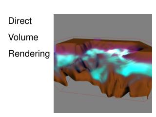
Direct Volume Rendering • Render volume without extracting any surfaces (DVR) • Map scalar values to optical properties(color, opacity) • Need optical model • Solve volume renderingintegral for viewing raysinto the volume R. Crawfis, Ohio State Univ.
Direct Rendering Pipeline I • Detection of Structures • Shading • Reconstruct (interpolate/filter) color/opacity • Composite • Final Image Validation (change parameters) R. Crawfis, Ohio State Univ.
Direct Rendering Pipeline ClassifyShade Reconstruct Visibilityorder Composite Validate R. Crawfis, Ohio State Univ.
Early Methods • Before 1988 • Did not consider transparency • did not consider sophisticated light transportation theory • were concerned with quick solutions • hence more or less applied to binary data R. Crawfis, Ohio State Univ.
Back-To-Front - Frieder et al 1985 • A viewing algorithm that traverses and renders the scene objects in order of decreasing distance from the observer. • Maybe derived from a standard -“Painters Algorithm” 1. 2. 3. R. Crawfis, Ohio State Univ.
Back-To-Front - Frieder et al 1985 • 2D • Start traversal at point farthest from the observer, • 2 orders • Either x or y can be innermost loop • If x is innermost, display order will be A, C, B, D • If y is innermost, display order will be C, A, D, B • Both result in the correct image! • If voxel (x,y) is (partially) obscured by voxel (x’,y’), then x <= x’ and y <= y’. So project (x,y) before (x’,y’) and the image will be correct R. Crawfis, Ohio State Univ.
Back-To-Front - Frieder et al 1985 • 3D • Axis traversal can still be done arbitrarily, 8 orders • Data can be read and rendered as slices • Note: voxel projection is NOT in order of strictly decreasing distance, so this is not the painter’s algorithm. • Perspective? R. Crawfis, Ohio State Univ.
Ray Casting • Goal: numerical approximation of the volume rendering integral • Resample volume at equispacedlocations along the ray • Reconstruct at continuouslocation via tri-linearinterpolation • Approximate integral R. Crawfis, Ohio State Univ.
Ray Tracing • “another” typical method from traditional graphics • Typically we only deal with primary rays -hence: ray-casting • a natural image-order technique • as opposed to surface graphics - how do we calculate the ray/surface intersection??? • Since we have no surfaces - we need to carefully step through the volume R. Crawfis, Ohio State Univ.
Ray Casting • Since we have no surfaces - we need to carefully step through the volume: a ray is cast into the volume, sampling the volume at certain intervals • The sampling intervals are usually equi-distant, but don’t have to be (e.g. importance sampling) • At each sampling location, a sample is interpolated / reconstructed from the grid voxels • popular filters are: nearest neighbor (box), trilinear (tent), Gaussian, cubic spline • Along the ray - what are we looking for? R. Crawfis, Ohio State Univ.
Basic Idea of Ray-casting Pipeline • Data are defined at the corners of each cell (voxel) • The data value inside the voxel is determined using interpolation (e.g. tri-linear) • Composite colors and opacities along the ray path • Can use other ray-traversal schemes as well c1 c2 c3 R. Crawfis, Ohio State Univ.
Evaluation = Compositing • “over” operator - Porter & Duff 1984 R. Crawfis, Ohio State Univ.
c= af*cf + (1 - af)*ab*cb a= af + (1 - af)*ab c= (0.54,0.4,0) a= 0.94 Compositing: Over Operator cf= (0,1,0) af= 0.4 cb= (1,0,0) ab= 0.9 R. Crawfis, Ohio State Univ.
1.0 Volumetric Ray Integration color opacity object (color, opacity) R. Crawfis, Ohio State Univ.
Interpolation Closest value Weighted average R. Crawfis, Ohio State Univ.
Tri-Linear Interpolation R. Crawfis, Ohio State Univ.
1.0 Interpolation Kernels volumetric compositing color opacity object (color, opacity) R. Crawfis, Ohio State Univ.
Interpolation Kernels interpolation kernel volumetric compositing color opacity color c = c s s(1 - ) + c opacity = s (1 - ) + 1.0 object (color, opacity) R. Crawfis, Ohio State Univ.
1.0 Interpolation Kernels interpolation kernel volumetric compositing color opacity object (color, opacity) R. Crawfis, Ohio State Univ.
Interpolation Kernels volumetric compositing color opacity 1.0 object (color, opacity) R. Crawfis, Ohio State Univ.
Interpolation Kernels volumetric compositing color opacity 1.0 object (color, opacity) R. Crawfis, Ohio State Univ.
Interpolation Kernels volumetric compositing color opacity 1.0 object (color, opacity) R. Crawfis, Ohio State Univ.
Interpolation Kernels volumetric compositing color opacity 1.0 object (color, opacity) R. Crawfis, Ohio State Univ.
Interpolation Kernels volumetric compositing color opacity object (color, opacity) R. Crawfis, Ohio State Univ.
Levoy - Pipeline Acquired values Data preparation Prepared values shading classification Voxel colors Voxel opacities Ray-tracing / resampling Ray-tracing / resampling Sample colors Sample opacities compositing Image Pixels R. Crawfis, Ohio State Univ.
Ray Marching • Use a 3D DDA algorithm to step through regular or rectilinear grids. R. Crawfis, Ohio State Univ.
Adaptive Ray Sampling[Hanrahan et al 92] • Sampling rate is adjusted to the significance of the traversed data R. Crawfis, Ohio State Univ.
Classification How do we obtain the emission and absorption values? scalar value s T(s) emission RGB absorption A R. Crawfis, Ohio State Univ.
Ray Traversal Schemes Intensity Max Average Accumulate First Depth R. Crawfis, Ohio State Univ.
Ray Traversal - First Intensity • First: extracts iso-surfaces (again!)done by Tuy&Tuy ’84 First Depth R. Crawfis, Ohio State Univ.
Ray Traversal - Average Intensity • Average: produces basically an X-ray picture Average Depth R. Crawfis, Ohio State Univ.
Ray Traversal - MIP Intensity • Max: Maximum Intensity Projectionused for Magnetic Resonance Angiogram Max Depth R. Crawfis, Ohio State Univ.
Maximum Intensity Projection (1) • No emission or absorption • Pixel value is maximum scalar value along the viewing ray • Advantage: no transfer function required • Drawback: misleading depth information • Works well for MRI data (esp. angiography) Maximum Smax Scalar value S s s0 ray R. Crawfis, Ohio State Univ.
Maximum Intensity Projection (2) Emission/Absorption MIP R. Crawfis, Ohio State Univ.