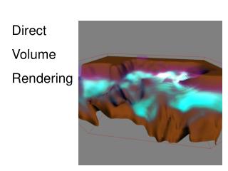
Direct Volume Rendering

1. Direct Volume Rendering

2. What is volume rendering? • Accumulate information along 1 dimension line through volume

3. Volume rendering vs. isosurfaces • No intermediate geometry • No thresholding needed • View dependent • Uses all data instead of just some • Fuzzy vs sharp appearance

4. Two General Methods Two general methods: • Image order: ray casting • Object order: splatting

5. Other methods (handwaving only!) • Texture slabs • Volume loaded into texture map memory of graphics card • “slab” between each pair of volume rendering slices • Pre-integration of volume rendering integral possible

6. Other methods, cont’d • Fourier volume rendering • Many 1D projections from unique angles • 1D Fourier transform interpolated to 2D array F(wx,wy) • Invert Fourier to recover original density function f(x,y)

7. The Volume Integral • B = ∫I D (cos ) e-∫D ds dt • : angle between I & E at each voxel on ray • B: cumulative attenuated info along ray • : decay constant • D ds: accumulated densities between voxel & light source I E Attenuate: to lessen the amount, force, magnitude, or value of

8. Image Order, color C, opacity  • Ray Casting • 3D density data (e.g., CAT scan) • 3D color C(x,y,z) • 3D opacity (x,y,z) • C(x,y,z) determined by gradient (“surface” normal) & lighting (independent of other volume voxels between the point & the light) • (x,y,z) determined by mapping density values to different types of tissue DVR

9. Raycast! • Raycast: combine c &  into C(R), color seen by ray R. K KC(R) =∑ C(R,k)  (R,k) (1 -  (R,j))k=0 j=k+1 (R,k) : kth voxel along ray C(R,0): color of background (back to front!) (R,0) = 1 (opaque background) For each pixel, shoot ray, calculate C(R)

10. Raycasting Variations/Issues • MIP- maximum intensity projectiongood for noisy data but lose differentiation of in front/behind - where does max lay? Single Ray Max intensity A Mean Intensity B Scalar value Distance along ray C C(R) = A or C(R) = B or C(R) = C, (distance to reach accumulated value)

11. More Variations/Issues 2. Sampling • Regular sampling • What is correct step size? Computation cost vs smoothness, may miss details • Cell intersection • What if ray enters near 90 degrees? • Bresenham method • Other issues covered in VTK text

12. More Variations/Issues • Parallel (easy for hardware!) vs. perspective projection( will image warp?) • Starting point for sampling Initial point of ray 1st intersection

13. More Variations/Issues • Data vs color • Calculate color at each vertex, then trilinear interpolate to sample • Use data at each vertex, trilinear interpolate to sample. THEN convert to color based on interpolated values • Early termination based on accumulated opacity

14. Object Order • For each voxel • Project (throw) voxel to projection screen • Apply filtering to ‘splat’, e.g. gaussian,proportional to distance from plane • Alpha blending • Splatting may be done • Front to back • Back to front

15. Object Order • Discrete process which produces holes on the periphery or when perspective projection gets extreme.! • Countered by distributing the energy across multiple pixels via a footprint table. All splats make a footprint and, using the table, adjustmentscan be made beforerendering. Note: Footprint is the same for each voxel when using parallel projection

16. Coherent Projection • Scanline algorithm • Much faster than splatting • for parallel projection • Scan converts the depth information behind each projected polygon. (Recall scan conversion: line-by-line, fill polygons) • Interpolated data and color samples used in raycasting can be accounted for by integrating the values at each scan converting step.