Random Variable and Probability Distribution

1. Random Variable and Probability Distribution

2. Outline of Lecture • Random Variable • Discrete Random Variable. • Continuous Random Variables. • Probability Distribution Function. • Discrete and Continuous. • PDF and PMF. • Expectation of Random Variables. • Propagation through Linear and Nonlinear model. • Multivariate Probability Density Functions. • Some Important Probability Distribution Functions.

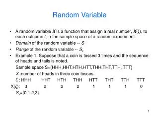
3. Random Variables • A random variables are functions that associate a numerical value to each outcome of an experiment. • Function values are real numbers and depend on “chance”. • The function that assigns value to each outcome is fixed and deterministic. • The randomness is due to the underlying randomness of the argument of the function X. • If we roll a pair of dice then the sum of two face values is a random variable. • Random numbers can be Discrete or Continuous. • Discrete: Countable Range. • Continuous: Uncountable Range.

4. Discrete Random Variables • A random variable X and the corresponding distribution are said to be discrete, if the number of values for which X has non-zero probability is finite. • Probability Mass Function of X: • Probability Distribution Function of x: • Properties of Distribution Function:

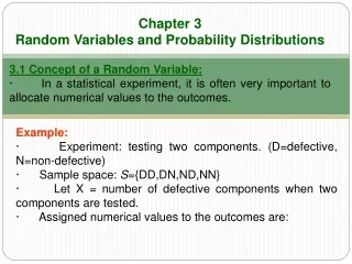
5. Examples • X denote the number of heads when a biased coin with probability of head p is tossed twice. • X can take value 0, 1 or 2. • X denote the random variable that is equal to sum of two fair dices. • Random variable can take any integral value between 1 and 12.

6. Continuous Random Variables and Distributions • X is a continuous random variable if there exists a non-negative function f(x) defined for real line having the property that • The integrand f(y) is called a probability density function. • Properties:

7. Continuous Random Variables and Distributions • Probability that a continuous random variable will assume any particular value is zero. • It does not mean that event will never occur. • Occur infrequently and its relative frequency will converge to zero. • f(a) large Probability mass is very dense. • f(a) small  Probability mass is not very dense. • f(a) is the measure of how likely it is that random variable will be near a.

8. a b Difference Between PDF and PMF • Probability density function does not defines a probability but probability density. • To obtain the probability we must integrate it in an interval. • Probability mass function gives the true probability. • It does not need to be integrate to obtain the probability. • Probability distribution function is either continuous or has a jump discontinuity. • Are they equal?

9. Statistical Characterization of Random Variables • Recall, a random number denote the numerical attribute assigned to an outcome of an experiment. • We can not be certain which value of X will be observed on a particular trial. • Will average of all the values will be same for two different set of trials? • Recall, probability approx. equal to relative frequency. • Approx. Np1 number of xi’s have value u1

10. Statistical Characterization of Random Variables • Expected Value: • The expected value of a discrete random variable, x is found by multiplying each value of random variable by its probability and then summing over all values of x. • Expected value is equivalent to center of mass concept. • That’s why name first moment also. • Body is perfectly balanced abt. Center of mass • The expectation value of x is the “balancing point” for the probability mass function of x • Expected value is equal to the point of symmetry in case of symmetric pmf/pdf.

11. Statistical Characterization of Random Variables • Law of Unconscious Statistician (LOTUS): We can take an expectation of any function of a random variable. • This balance point is the value expected for g(x) for all possible repetitions of the experiment involving the random variable x. • Expected value of a continuous density function f(x), is given by

12. Example • Let us assume that we have agreed to pay $1 for each dot showing when a pair of dice is thrown. We are interested in knowing, how much we would lose on the average? • Average amount we pay= (($2x1)+($3x2)+……+($12x1))/36=$7 • E(x)=$2(1/36)+$3(2/36)+……….+$12(1/36)=$7

13. Example (Continue…) • Let us assume that we had agreed to pay an amount equal to the squares of the sum of the dots showing on a throw of dice. • What would be the average loss this time? • Will it be ($7)2=$49.00? • Actually, now we are interested in calculating E[x2]. • E[x2]=($2)2(1/36)+……….+($12)2(1/36)=$54.83  $49 • This result also emphasized that (E[x])2  E[x2]

14. Expectation Rules • Rule 1: E[k]=k; where k is a constant • Rule 2: E[kx] = kE[x]. • Rule 3: E[x  y] = E[x]  E[y]. • Rule 4: If x and y are independent E[xy] = E[x]E[y] • Rule 5: V[k] = 0; where k is a constant • Rule 6: V[kx] = k2V[x]

15. Variance of Random Variable • Variance of random variable, x is defined as This result is also known as “Parallel Axis Theorem”

16. Propagation of moments and density function through linear models • y=ax+b • Given:  = E[x] and 2 = V[x] • To find: E[y] and V[y] E[y] = E[ax]+E[b] = aE[x]+b = a+b V[y] = V[ax]+V[b] = a2V[x]+0 = a2 2 • Let us define Here, a = 1/  and b = - /  Therefore, E[z] = 0 and V[z] = 1 z is generally known as “Standardized variable”

17. Propagation of moments and density function through non-linear models • If x is a random variable with probability density function p(x) and y = f(x) is a one to one transformation that is differentiable for all x then the probability function of y is given by • p(y)=p(x)|J|-1, for all x given by x=f-1(y) • where J is the determinant of Jacobian matrix J. • Example: NOTE: for each value of y there are two values of x. and p(y) = 0, otherwise We can also show that

18. Random Variables • One random number depicts one physical phenomenon. • Web server. • Just an extension to random variable • A vector random variable X is a function that assigns a vector of real number to each outcome in the sample space. • e.g. Sample Space = Set of People. • Random vector=[X=weight, Y=height of a person]. • A random point (X,Y) has more information than X or Y. • It describes the joint behavior of X and Y. • The joint probability distribution function: • What Happens:

19. Random Vectors • Joint Probability Functions: • Joint Probability Distribution Function: • Joint Probability Density Function: • Marginal Probability Functions: A marginal probability functions are obtained by integrating out the variables that are of no interest.

20. Multivariate Expectations What abt. g(X,Y)=X+Y

21. Multivariate Expectations • Mean Vector: • Expected value of g(x1,x2,…….,xn) is given by • Covariance Matrix: R is the correlation matrix

22. Covariance Matrix • Covariance matrix indicates the tendency of each pair of dimensions in random vector to vary together i.e. “co-vary”. • Properties of covariance matrix: • Covariance matrix is square. • Covariance matrix is always +ive definite i.e. xTPx > 0. • Covariance matrix is symmetric i.e. P = PT. • If xi and xj tends to increase together then Pij > 0. • If xi and xj are uncorrelated then Pij = 0.

23. Independent Variables • Recall, two random variables are said to be independent if knowing values of one tells you nothing about the other variable. • Joint probability density function is product of the marginal probability density functions. • Cov(X,Y)=0 if X and Y are independent. • E(XY)=E(X)E(Y). • Two variables are said to be uncorrelated if cov(X,Y)=0. • Independent variables are uncorrelated but vice versa is not true. • Cov(X,Y)=0Integral=0. • It tells us that distribution is balanced in some way but says nothing abt. Distribution values. • Example: (X,Y) uniformly distributed on unit circle.

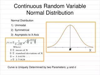
24. 0.3413 0.3413 0.1359 0.1359 -2 -  + +2 Gaussian or Normal Distribution • The normal distribution is the most widely known and used distribution in the field of statistics. • Many natural phenomena can be approximated by Normal distribution. • Central Limit Theorem: • The central limit theorem states that given a distribution with a mean  and variance 2, the sampling distribution of the mean approaches a normal distribution with a mean  and a variance 2/N as N, the sample size increases. • Normal Density Function:

25. Multivariate Normal Distribution • Multivariate Gaussian Density Function: • How to find equal probability surface? • More ever one is interested to find the probability of x lies inside the quadratic hyper surface • For example what is the probability of lying inside 1-σ ellipsoid.

26. n\c Curse of Dimensionality Multivariate Normal Distribution • Yi represents coordinates based on Cartesian principal axis system and σ2i is the variance along the principal axes. • Probability of lying inside 1σ,2σ or 3σ ellipsoid decreases with increase in dimensionality.

27. Summary of Probability Distribution Functions A distribution is skewed if it has most of its values either to the right or to the left of its mean

28. Properties of Estimators • Unbiasedness • On average the value of parameter being estimated is equal to true value. • Efficiency • Have a relatively small variance. • The values of parameters being estimated should not vary with samples. • Sufficiency • Use as much as possible information available from the samples. • Consistency • As the sample size increases, the estimated value approaches the true value.